MFML Week 4: First nn.Module Classifier

Multi-class classification with IrisDataset

Open In Colab

Learning Objectives

Use CrossEntropyLoss for multi-class classification
Understand why class labels must be long (integer) tensors
Compute classification accuracy and visualize a confusion matrix

Setup

!pip install git+https://github.com/ECLIPSE-Lab/Ai4MatLectures.git "mdsdata>=0.1.5"

import torch
import torch.nn as nn
from torch.utils.data import DataLoader, random_split
from ai4mat.datasets import IrisDataset
import matplotlib.pyplot as plt
import numpy as np

1. Load the Data

dataset = IrisDataset()
print(f"Dataset size: {len(dataset)}")
x0, y0 = dataset[0]
print(f"Sample x shape: {x0.shape}, dtype: {x0.dtype}")
print(f"Sample y: {y0}, dtype: {y0.dtype}")
print(f"Number of classes: {len(torch.unique(torch.tensor([dataset[i][1] for i in range(len(dataset))])))}")

Dataset size: 150
Sample x shape: torch.Size([4]), dtype: torch.float32
Sample y: 0, dtype: torch.int64
Number of classes: 3

# Visualize pairwise scatter of first two features
X_all = torch.stack([dataset[i][0] for i in range(len(dataset))])
y_all = torch.tensor([dataset[i][1] for i in range(len(dataset))])

feature_names = ["Sepal length", "Sepal width", "Petal length", "Petal width"]
class_names = ["Setosa", "Versicolor", "Virginica"]
colors = ["tab:blue", "tab:orange", "tab:green"]

fig, axes = plt.subplots(1, 2, figsize=(10, 4))
for cls in range(3):
    mask = y_all == cls
    axes[0].scatter(X_all[mask, 0], X_all[mask, 1], label=class_names[cls], alpha=0.7)
    axes[1].scatter(X_all[mask, 2], X_all[mask, 3], label=class_names[cls], alpha=0.7)

axes[0].set_xlabel(feature_names[0])
axes[0].set_ylabel(feature_names[1])
axes[0].set_title("Features 0 vs 1")
axes[0].legend()

axes[1].set_xlabel(feature_names[2])
axes[1].set_ylabel(feature_names[3])
axes[1].set_title("Features 2 vs 3")
axes[1].legend()

plt.tight_layout()
plt.show()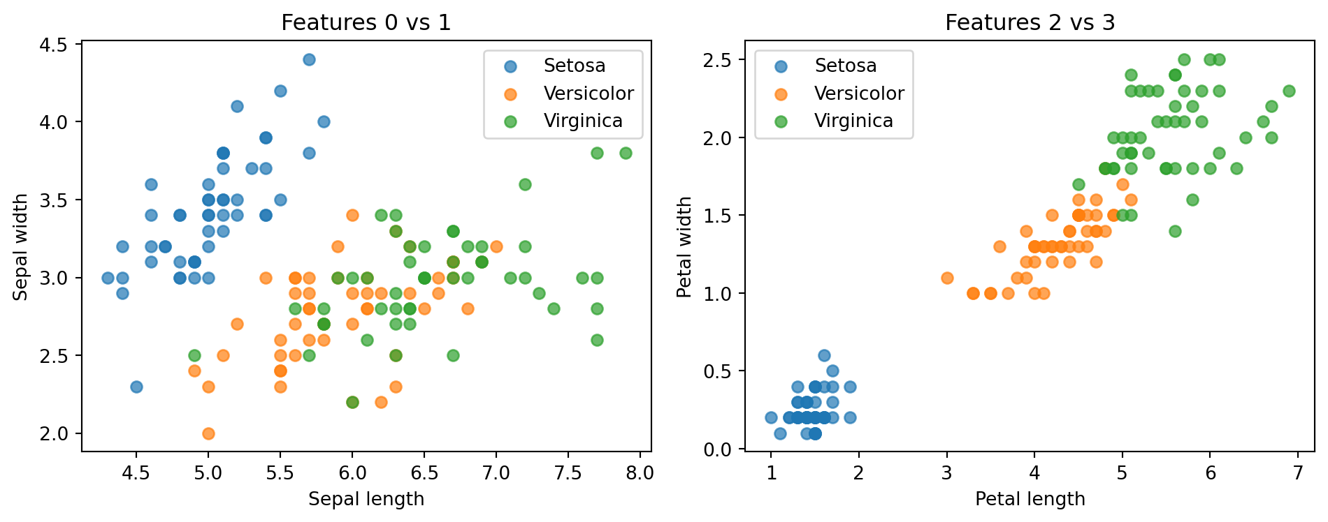

2. Train/Val Split

n_train = int(0.8 * len(dataset))
n_val = len(dataset) - n_train
train_ds, val_ds = random_split(dataset, [n_train, n_val])

train_loader = DataLoader(train_ds, batch_size=32, shuffle=True)
val_loader   = DataLoader(val_ds,   batch_size=32, shuffle=False)
print(f"Train: {n_train} | Val: {n_val}")

Train: 120 | Val: 30

3. Define the Model

# CrossEntropyLoss expects raw logits (no softmax) as input
# and long integer class indices as targets
model = nn.Sequential(
    nn.Linear(4, 16),
    nn.ReLU(),
    nn.Linear(16, 3)
)
print(model)
print(f"Parameters: {sum(p.numel() for p in model.parameters())}")

Sequential(
  (0): Linear(in_features=4, out_features=16, bias=True)
  (1): ReLU()
  (2): Linear(in_features=16, out_features=3, bias=True)
)
Parameters: 131

4. Training Loop

criterion = nn.CrossEntropyLoss()
optimizer = torch.optim.Adam(model.parameters(), lr=1e-3)

train_losses, val_losses = [], []
train_accs, val_accs = [], []

def accuracy(logits, labels):
    preds = logits.argmax(dim=1)
    return (preds == labels).float().mean().item()

for epoch in range(100):
    model.train()
    epoch_loss, epoch_acc = 0.0, 0.0
    for x_batch, y_batch in train_loader:
        optimizer.zero_grad()
        logits = model(x_batch)
        loss = criterion(logits, y_batch)
        loss.backward()
        optimizer.step()
        epoch_loss += loss.item() * len(x_batch)
        epoch_acc  += accuracy(logits, y_batch) * len(x_batch)
    train_losses.append(epoch_loss / n_train)
    train_accs.append(epoch_acc / n_train)

    model.eval()
    val_loss, val_acc = 0.0, 0.0
    with torch.no_grad():
        for x_batch, y_batch in val_loader:
            logits = model(x_batch)
            val_loss += criterion(logits, y_batch).item() * len(x_batch)
            val_acc  += accuracy(logits, y_batch) * len(x_batch)
    val_losses.append(val_loss / n_val)
    val_accs.append(val_acc / n_val)

fig, axes = plt.subplots(1, 2, figsize=(12, 4))
axes[0].plot(train_losses, label='Train')
axes[0].plot(val_losses, label='Val')
axes[0].set_xlabel("Epoch"); axes[0].set_ylabel("Cross-Entropy Loss")
axes[0].set_title("Loss Curve"); axes[0].legend()

axes[1].plot(train_accs, label='Train')
axes[1].plot(val_accs, label='Val')
axes[1].set_xlabel("Epoch"); axes[1].set_ylabel("Accuracy")
axes[1].set_title("Accuracy Curve"); axes[1].legend()

plt.tight_layout()
plt.show()
print(f"Final val accuracy: {val_accs[-1]:.3f}")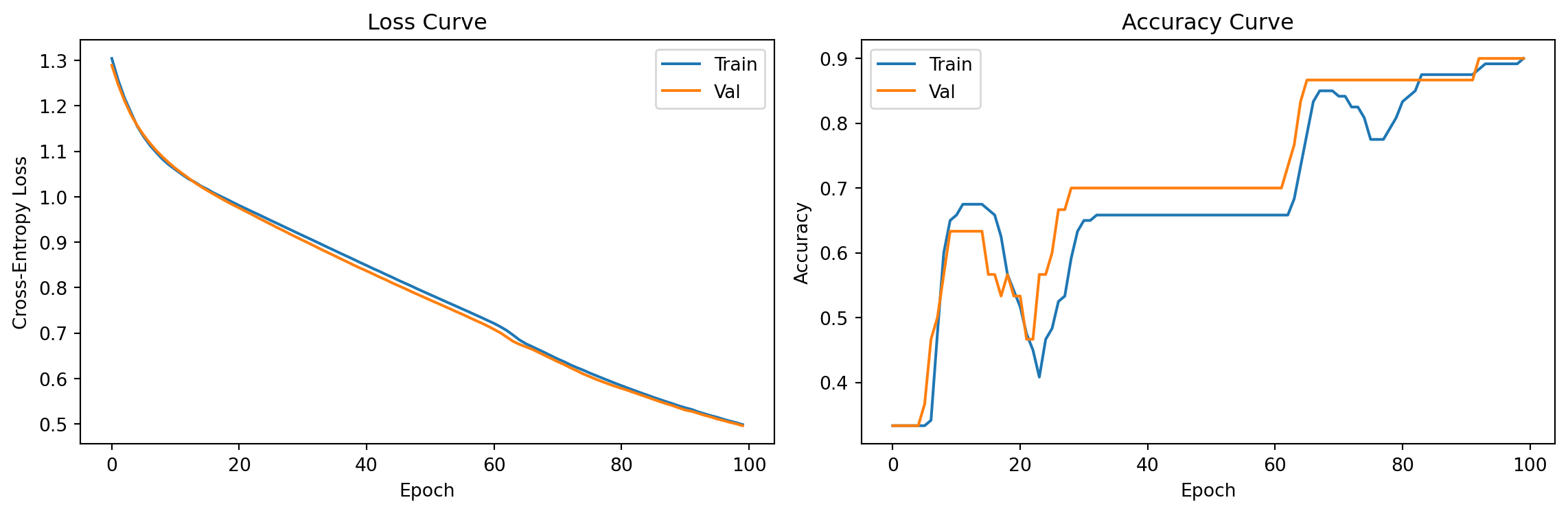

Final val accuracy: 0.900

5. Evaluation

# Compute predictions on full dataset
model.eval()
with torch.no_grad():
    logits_all = model(X_all)
    preds_all = logits_all.argmax(dim=1)

# Build confusion matrix manually (no sklearn)
n_classes = 3
conf_matrix = torch.zeros(n_classes, n_classes, dtype=torch.long)
for true, pred in zip(y_all, preds_all):
    conf_matrix[true.item(), pred.item()] += 1

print("Confusion Matrix (rows=true, cols=predicted):")
print(conf_matrix.numpy())
print(f"\nOverall accuracy: {(preds_all == y_all).float().mean().item():.3f}")

Confusion Matrix (rows=true, cols=predicted):
[[50  0  0]
 [ 0 34 16]
 [ 0  0 50]]

Overall accuracy: 0.893

# Visualize confusion matrix
fig, ax = plt.subplots(figsize=(5, 4))
im = ax.imshow(conf_matrix.numpy(), cmap='Blues')
plt.colorbar(im, ax=ax)
ax.set_xticks(range(n_classes)); ax.set_xticklabels(class_names)
ax.set_yticks(range(n_classes)); ax.set_yticklabels(class_names)
ax.set_xlabel("Predicted")
ax.set_ylabel("True")
ax.set_title("Confusion Matrix")

for i in range(n_classes):
    for j in range(n_classes):
        ax.text(j, i, conf_matrix[i, j].item(),
                ha='center', va='center', color='black', fontsize=12)

plt.tight_layout()
plt.show()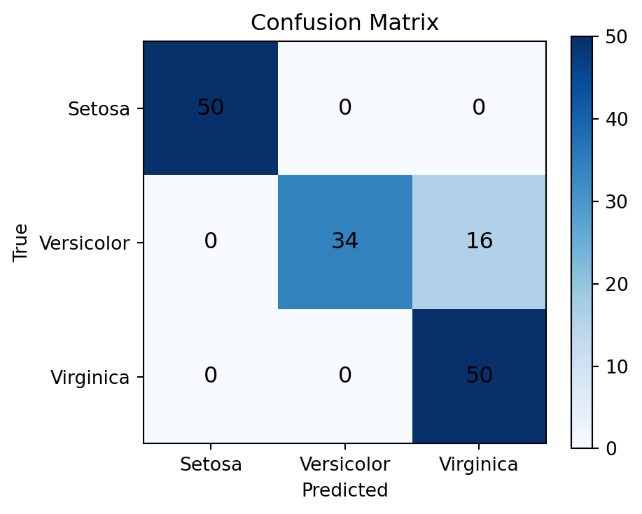

Exercises

Try nn.Linear(4, 3) directly (no hidden layer) — how does the final accuracy change? Why does the hidden layer help?
Plot learning curves for both train and val accuracy on the same axes. At what epoch does validation accuracy plateau?
Change batch_size from 32 to 4. How does the training curve change? Why is small batch size sometimes called “noisy” optimization?