MFML Week 5: Manual Backprop

Understanding autograd with DigitsDataset

Open In Colab

Learning Objectives

Connect the chain rule to .grad tensors populated by .backward()
Implement manual gradient computation for a single linear layer
Verify that manual gradients match PyTorch autograd results

Setup

!pip install git+https://github.com/ECLIPSE-Lab/Ai4MatLectures.git "mdsdata>=0.1.5"

import torch
import torch.nn as nn
from torch.utils.data import DataLoader, random_split
from ai4mat.datasets import DigitsDataset
import matplotlib.pyplot as plt
import numpy as np

1. Load the Data

dataset = DigitsDataset()
print(f"Dataset size: {len(dataset)}")
x0, y0 = dataset[0]
print(f"Sample x shape: {x0.shape}, dtype: {x0.dtype}")
print(f"Sample y: {y0}, dtype: {y0.dtype}")

n_classes = len(torch.unique(torch.tensor([dataset[i][1] for i in range(len(dataset))])))
print(f"Number of classes: {n_classes}")

Dataset size: 5620
Sample x shape: torch.Size([64]), dtype: torch.float32
Sample y: 0, dtype: torch.int64
Number of classes: 10

# Visualize a few digit images (each sample is a flat 64-dim vector from 8x8 images)
fig, axes = plt.subplots(2, 8, figsize=(14, 4))
for i, ax in enumerate(axes.flat):
    img = dataset[i][0].reshape(8, 8).numpy()
    ax.imshow(img, cmap='gray_r', vmin=0, vmax=1)
    ax.set_title(f"y={dataset[i][1].item()}", fontsize=8)
    ax.axis('off')
plt.suptitle("Sample digit images (8×8 pixels, flattened to 64 features)")
plt.tight_layout()
plt.show()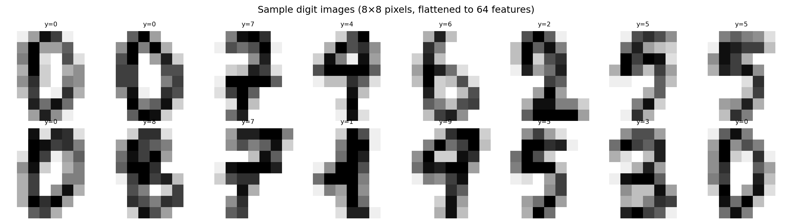

2. Train/Val Split

n_train = int(0.8 * len(dataset))
n_val = len(dataset) - n_train
train_ds, val_ds = random_split(dataset, [n_train, n_val])

train_loader = DataLoader(train_ds, batch_size=64, shuffle=True)
val_loader   = DataLoader(val_ds,   batch_size=64, shuffle=False)
print(f"Train: {n_train} | Val: {n_val}")

Train: 4496 | Val: 1124

3. Manual Gradient Verification

Before training, let’s verify that PyTorch’s autograd produces correct gradients.

For a single linear layer y = W x + b followed by MSE loss, the analytical gradient is:

dL/dW = (2/n) * (y_pred - y_true)^T * x (for MSE: L = mean((Wx+b - y)^2))

# Toy example: single linear layer, batch of 4 samples
torch.manual_seed(42)
W = torch.randn(3, 4, requires_grad=True)  # output_dim x input_dim
b = torch.zeros(3, requires_grad=True)

x_toy = torch.randn(4, 4)   # batch_size x input_dim
y_toy = torch.randn(4, 3)   # batch_size x output_dim (regression target)

# Forward pass
y_pred = x_toy @ W.T + b    # (4, 3)
loss = ((y_pred - y_toy) ** 2).mean()

# Autograd backward
loss.backward()
autograd_dW = W.grad.clone()

# Manual gradient: dL/dW = (2/n) * (y_pred - y_toy)^T @ x
# Note: mean over n*output_dim elements
n_total = y_toy.numel()
manual_dW = (2.0 / n_total) * (y_pred.detach() - y_toy).T @ x_toy

print("Autograd dW (first row):", autograd_dW[0].numpy())
print("Manual  dW (first row):", manual_dW[0].numpy())
print(f"\nMax absolute difference: {(autograd_dW - manual_dW).abs().max().item():.2e}")
print("Gradients match!" if torch.allclose(autograd_dW, manual_dW, atol=1e-5) else "Mismatch!")

Autograd dW (first row): [0.35887453 0.18204454 0.82238907 0.02623338]
Manual  dW (first row): [0.35887453 0.18204454 0.82238907 0.02623338]

Max absolute difference: 0.00e+00
Gradients match!

# Inspect the computation graph
print("loss.grad_fn:", loss.grad_fn)
print("  └─", loss.grad_fn.next_functions[0][0])
print("     └─", loss.grad_fn.next_functions[0][0].next_functions[0][0])
print("        └─ ... (AddmmBackward0 → MmBackward0 → AccumulateGrad)")
print()
print("The chain rule flows backward through these nodes,")
print("accumulating gradients into W.grad and b.grad.")

loss.grad_fn: <MeanBackward0 object at 0x7bc9b4340eb0>
  └─ <PowBackward0 object at 0x7bc9b4341d50>
     └─ <SubBackward0 object at 0x7bc9b4340eb0>
        └─ ... (AddmmBackward0 → MmBackward0 → AccumulateGrad)

The chain rule flows backward through these nodes,
accumulating gradients into W.grad and b.grad.

4. Define the Model

model = nn.Sequential(
    nn.Linear(64, 32),
    nn.ReLU(),
    nn.Linear(32, 10)
)
print(model)
print(f"Total parameters: {sum(p.numel() for p in model.parameters())}")

Sequential(
  (0): Linear(in_features=64, out_features=32, bias=True)
  (1): ReLU()
  (2): Linear(in_features=32, out_features=10, bias=True)
)
Total parameters: 2410

5. Training Loop

criterion = nn.CrossEntropyLoss()
optimizer = torch.optim.Adam(model.parameters(), lr=1e-3)

train_losses, val_losses = [], []
train_accs, val_accs = [], []

def accuracy(logits, labels):
    return (logits.argmax(dim=1) == labels).float().mean().item()

for epoch in range(30):
    model.train()
    ep_loss, ep_acc = 0.0, 0.0
    for x_batch, y_batch in train_loader:
        optimizer.zero_grad()
        logits = model(x_batch)
        loss = criterion(logits, y_batch)
        loss.backward()
        optimizer.step()
        ep_loss += loss.item() * len(x_batch)
        ep_acc  += accuracy(logits, y_batch) * len(x_batch)
    train_losses.append(ep_loss / n_train)
    train_accs.append(ep_acc / n_train)

    model.eval()
    v_loss, v_acc = 0.0, 0.0
    with torch.no_grad():
        for x_batch, y_batch in val_loader:
            logits = model(x_batch)
            v_loss += criterion(logits, y_batch).item() * len(x_batch)
            v_acc  += accuracy(logits, y_batch) * len(x_batch)
    val_losses.append(v_loss / n_val)
    val_accs.append(v_acc / n_val)

fig, axes = plt.subplots(1, 2, figsize=(12, 4))
axes[0].plot(train_losses, label='Train'); axes[0].plot(val_losses, label='Val')
axes[0].set_xlabel("Epoch"); axes[0].set_ylabel("Loss"); axes[0].set_title("Loss"); axes[0].legend()
axes[1].plot(train_accs, label='Train'); axes[1].plot(val_accs, label='Val')
axes[1].set_xlabel("Epoch"); axes[1].set_ylabel("Accuracy"); axes[1].set_title("Accuracy"); axes[1].legend()
plt.tight_layout()
plt.show()
print(f"Final val accuracy: {val_accs[-1]:.3f}")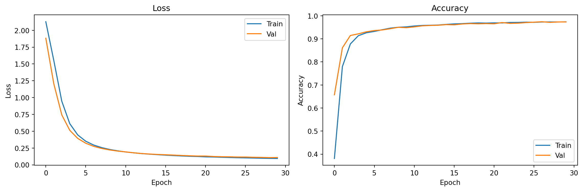

Final val accuracy: 0.973

6. Inspect Gradients After Backward

# Run one forward+backward pass and inspect gradients
x_sample, y_sample = next(iter(train_loader))
optimizer.zero_grad()
logits = model(x_sample)
loss = criterion(logits, y_sample)
loss.backward()

for name, param in model.named_parameters():
    print(f"{name:30s} grad norm: {param.grad.norm():.4f}")

0.weight                       grad norm: 0.3368
0.bias                         grad norm: 0.0945
2.weight                       grad norm: 0.4265
2.bias                         grad norm: 0.0517

Exercises

What is loss.grad_fn? Follow the chain back 3 steps by accessing .next_functions. What does each node represent?
Set requires_grad=False on the first layer’s weights: model[0].weight.requires_grad = False. What happens to training speed and final accuracy?
Try a deeper network by adding a nn.Linear(64, 64), nn.ReLU() layer at the start. Does validation accuracy improve?