MFML Week 7: Overfitting and Regularization

Bias-variance tradeoff with IsingDataset (light)

Open In Colab

Learning Objectives

Observe overfitting via train/val loss divergence for different model sizes
Understand the bias-variance tradeoff empirically
Apply L2 regularization via weight_decay in the optimizer

Setup

!pip install git+https://github.com/ECLIPSE-Lab/Ai4MatLectures.git "mdsdata>=0.1.5"

import torch
import torch.nn as nn
from torch.utils.data import DataLoader, random_split
from ai4mat.datasets import IsingDataset
import matplotlib.pyplot as plt

1. Load the Data

dataset = IsingDataset(size='light')
print(f"Dataset size: {len(dataset)}")
x0, y0 = dataset[0]
print(f"Sample x shape: {x0.shape}, dtype: {x0.dtype}")
print(f"Sample y: {y0}, dtype: {y0.dtype}")
print(f"Classes: {torch.unique(torch.tensor([dataset[i][1] for i in range(len(dataset))])).tolist()}")

Dataset size: 5000
Sample x shape: torch.Size([1, 16, 16]), dtype: torch.float32
Sample y: 1, dtype: torch.int64
Classes: [0, 1]

# Visualize a few Ising configurations
fig, axes = plt.subplots(2, 6, figsize=(14, 5))
label_names = {0: "Disordered (T > Tc)", 1: "Ordered (T < Tc)"}
for i, ax in enumerate(axes.flat):
    img = dataset[i][0].squeeze().numpy()
    ax.imshow(img, cmap='gray', vmin=0, vmax=1)
    ax.set_title(f"y={dataset[i][1].item()}", fontsize=8)
    ax.axis('off')
plt.suptitle("Ising spin configurations (16×16)")
plt.tight_layout()
plt.show()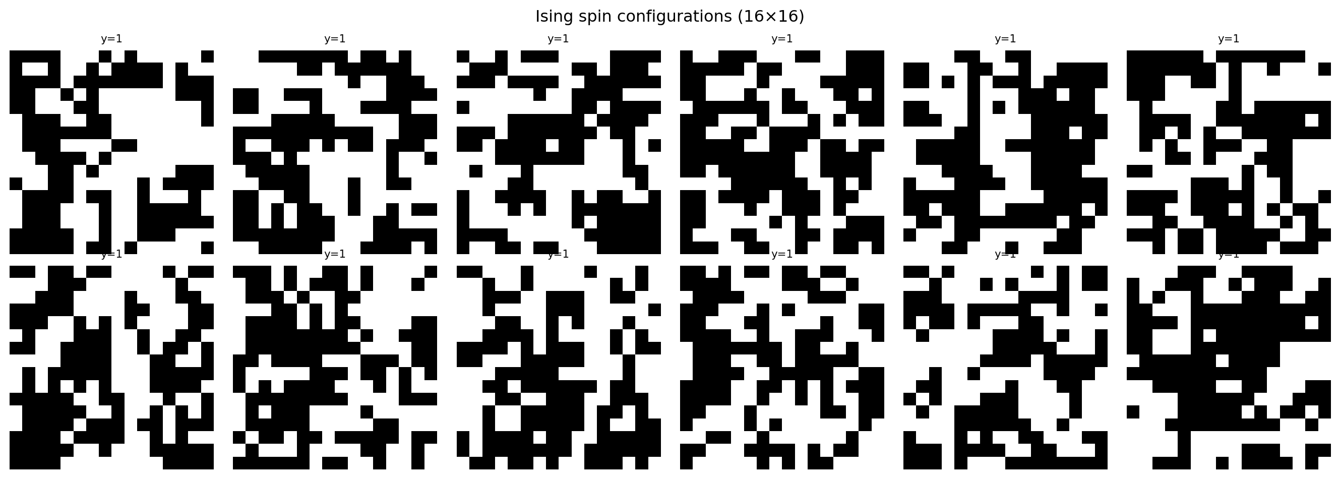

2. Train/Val Split

n_train = int(0.8 * len(dataset))
n_val = len(dataset) - n_train
train_ds, val_ds = random_split(dataset, [n_train, n_val])

train_loader = DataLoader(train_ds, batch_size=64, shuffle=True)
val_loader   = DataLoader(val_ds,   batch_size=64, shuffle=False)
print(f"Train: {n_train} | Val: {n_val}")

Train: 4000 | Val: 1000

3. Three Model Variants

We define three models of increasing capacity to illustrate the bias-variance tradeoff.

def make_underfit():
    """Underfitting: too few parameters to capture the decision boundary."""
    return nn.Sequential(
        nn.Flatten(),
        nn.Linear(256, 2)
    )

def make_goodfit():
    """Good fit: moderate capacity, good generalization."""
    return nn.Sequential(
        nn.Flatten(),
        nn.Linear(256, 64),
        nn.ReLU(),
        nn.Linear(64, 2)
    )

def make_overfit():
    """Overfitting: too many parameters, memorizes training data."""
    return nn.Sequential(
        nn.Flatten(),
        nn.Linear(256, 256),
        nn.ReLU(),
        nn.Linear(256, 256),
        nn.ReLU(),
        nn.Linear(256, 2)
    )

for name, fn in [("Underfit", make_underfit), ("Good fit", make_goodfit), ("Overfit", make_overfit)]:
    m = fn()
    n_params = sum(p.numel() for p in m.parameters())
    print(f"{name:12s}: {n_params:>7,} parameters")

Underfit    :     514 parameters
Good fit    :  16,578 parameters
Overfit     : 132,098 parameters

4. Training Loop

def train_model(model, train_loader, val_loader, n_train, n_val,
                lr=1e-3, weight_decay=0.0, epochs=50):
    criterion = nn.CrossEntropyLoss()
    optimizer = torch.optim.Adam(model.parameters(), lr=lr, weight_decay=weight_decay)
    train_losses, val_losses = [], []

    for epoch in range(epochs):
        model.train()
        ep_loss = 0.0
        for x_batch, y_batch in train_loader:
            optimizer.zero_grad()
            loss = criterion(model(x_batch), y_batch)
            loss.backward()
            optimizer.step()
            ep_loss += loss.item() * len(x_batch)
        train_losses.append(ep_loss / n_train)

        model.eval()
        v_loss = 0.0
        with torch.no_grad():
            for x_batch, y_batch in val_loader:
                v_loss += criterion(model(x_batch), y_batch).item() * len(x_batch)
        val_losses.append(v_loss / n_val)

    return train_losses, val_losses

# Train all three models
torch.manual_seed(0)
results = {}
for name, fn in [("Underfit", make_underfit), ("Good fit", make_goodfit), ("Overfit", make_overfit)]:
    model = fn()
    tl, vl = train_model(model, train_loader, val_loader, n_train, n_val)
    results[name] = (tl, vl)
    print(f"{name:12s} — final train loss: {tl[-1]:.4f}, val loss: {vl[-1]:.4f}")

Underfit     — final train loss: 0.6691, val loss: 0.7331
Good fit     — final train loss: 0.0023, val loss: 0.2267
Overfit      — final train loss: 0.0000, val loss: 0.3630

5. Compare Learning Curves

fig, axes = plt.subplots(1, 3, figsize=(15, 4))
colors = {'train': 'tab:blue', 'val': 'tab:orange'}

for ax, (name, (tl, vl)) in zip(axes, results.items()):
    ax.plot(tl, label='Train', color=colors['train'])
    ax.plot(vl, label='Val',   color=colors['val'])
    ax.set_title(name)
    ax.set_xlabel("Epoch")
    ax.set_ylabel("Cross-Entropy Loss")
    ax.legend()
    ax.set_ylim(0, max(max(tl), max(vl)) * 1.1)

plt.suptitle("Bias-Variance Tradeoff: Train vs Val Loss", fontsize=13)
plt.tight_layout()
plt.show()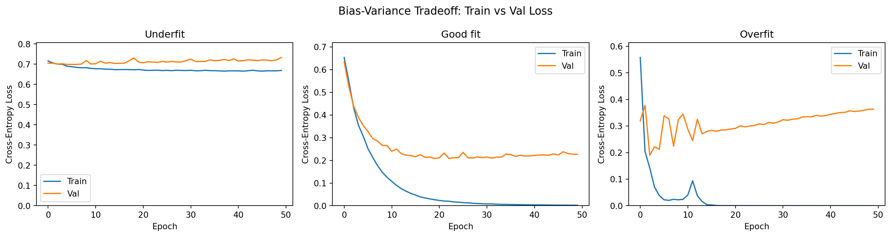

6. Regularization with Weight Decay

The overfitting model can be tamed by adding L2 regularization (weight_decay in Adam).

torch.manual_seed(0)
overfit_model_reg = make_overfit()
tl_reg, vl_reg = train_model(overfit_model_reg, train_loader, val_loader,
                              n_train, n_val, weight_decay=1e-4)

overfit_tl, overfit_vl = results["Overfit"]

plt.figure(figsize=(8, 4))
plt.plot(overfit_tl, '--', color='tab:blue',   label='Overfit — train (no reg)')
plt.plot(overfit_vl, '--', color='tab:orange', label='Overfit — val (no reg)')
plt.plot(tl_reg,     '-',  color='tab:blue',   label='Overfit — train (weight_decay=1e-4)')
plt.plot(vl_reg,     '-',  color='tab:orange', label='Overfit — val (weight_decay=1e-4)')
plt.xlabel("Epoch")
plt.ylabel("Cross-Entropy Loss")
plt.title("Effect of L2 Regularization on Overfit Model")
plt.legend(fontsize=8)
plt.tight_layout()
plt.show()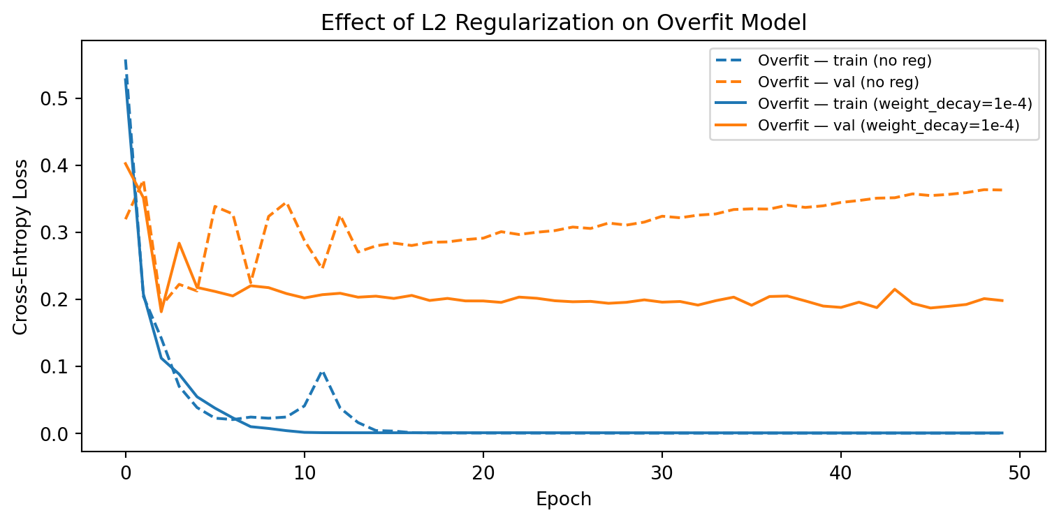

Exercises

At what model size (number of parameters) does overfitting first appear? Train a model with one extra layer in the “Good fit” config and observe the learning curves.
Try weight_decay=1e-2 vs 1e-4 vs 0 for the overfit model. How does the gap between train and val loss change?
Add nn.Dropout(0.5) after each nn.ReLU() in the overfit model. Does dropout reduce overfitting as effectively as weight decay?