!pip install git+https://github.com/ECLIPSE-Lab/Ai4MatLectures.git "mdsdata>=0.1.5"MFML Week 10: Convolutional Autoencoder
Unsupervised representation learning with IsingDataset (full)
![]()
Learning Objectives
- Build an encoder-decoder architecture with convolutional layers
- Train with pixel-wise reconstruction loss (MSE)
- Visualize the 2D latent space and connect its structure to physical labels
Setup
import torch
import torch.nn as nn
from torch.utils.data import DataLoader, random_split
from ai4mat.datasets import IsingDataset
import matplotlib.pyplot as plt
import numpy as np
1. Load the Data
dataset = IsingDataset(size='full')
print(f"Dataset size: {len(dataset)}")
x0, y0 = dataset[0]
print(f"Sample x shape: {x0.shape}, dtype: {x0.dtype}")
print(f"Sample y: {y0} (0=disordered T>Tc, 1=ordered T<Tc)")
Dataset size: 5000
Sample x shape: torch.Size([1, 64, 64]), dtype: torch.float32
Sample y: 0 (0=disordered T>Tc, 1=ordered T<Tc)fig, axes = plt.subplots(2, 5, figsize=(14, 6))
for i, ax in enumerate(axes.flat):
img = dataset[i * 500][0].squeeze().numpy()
label = dataset[i * 500][1].item()
ax.imshow(img, cmap='gray', vmin=0, vmax=1)
ax.set_title(f"{'Ordered' if label==1 else 'Disordered'}", fontsize=8)
ax.axis('off')
plt.suptitle("Ising spin configurations (64×64)")
plt.tight_layout()
plt.show()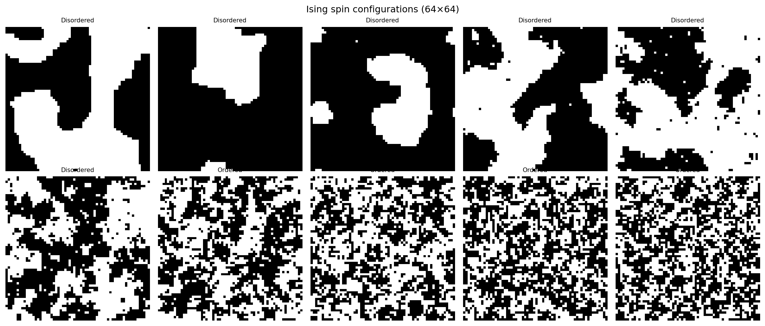
2. Train/Val Split
n_train = int(0.8 * len(dataset))
n_val = len(dataset) - n_train
train_ds, val_ds = random_split(dataset, [n_train, n_val])

train_loader = DataLoader(train_ds, batch_size=64, shuffle=True)
val_loader   = DataLoader(val_ds,   batch_size=64, shuffle=False)
print(f"Train: {n_train} | Val: {n_val}")
Train: 4000 | Val: 10003. Define the Autoencoder
class ConvAutoencoder(nn.Module):
    def __init__(self, latent_dim=2):
        super().__init__()
        self.encoder = nn.Sequential(
            nn.Conv2d(1, 16, 3, stride=2, padding=1),   # 32x32
            nn.ReLU(),
            nn.Conv2d(16, 32, 3, stride=2, padding=1),  # 16x16
            nn.ReLU(),
            nn.Flatten(),
            nn.Linear(32 * 16 * 16, latent_dim)
        )
        self.decoder = nn.Sequential(
            nn.Linear(latent_dim, 32 * 16 * 16),
            nn.ReLU(),
            nn.Unflatten(1, (32, 16, 16)),
            nn.ConvTranspose2d(32, 16, 3, stride=2, padding=1, output_padding=1),  # 32x32
            nn.ReLU(),
            nn.ConvTranspose2d(16, 1, 3, stride=2, padding=1, output_padding=1),   # 64x64
            nn.Sigmoid()
        )

    def forward(self, x):
        z = self.encoder(x)
        return self.decoder(z), z

model = ConvAutoencoder(latent_dim=2)
n_params = sum(p.numel() for p in model.parameters())
print(f"Autoencoder parameters: {n_params:,}")

# Test forward pass
x_test = torch.randn(4, 1, 64, 64)
x_recon, z = model(x_test)
print(f"Input shape:       {x_test.shape}")
print(f"Latent code shape: {z.shape}")
print(f"Output shape:      {x_recon.shape}")
Autoencoder parameters: 50,531
Input shape: torch.Size([4, 1, 64, 64])
Latent code shape: torch.Size([4, 2])
Output shape: torch.Size([4, 1, 64, 64])4. Training Loop
criterion = nn.MSELoss()
optimizer = torch.optim.Adam(model.parameters(), lr=1e-3)

train_losses, val_losses = [], []

for epoch in range(20):
    model.train()
    ep_loss = 0.0
    for x_batch, _ in train_loader:   # labels not used — unsupervised!
        optimizer.zero_grad()
        x_recon, _ = model(x_batch)
        loss = criterion(x_recon, x_batch)
        loss.backward()
        optimizer.step()
        ep_loss += loss.item() * len(x_batch)
    train_losses.append(ep_loss / n_train)

    model.eval()
    v_loss = 0.0
    with torch.no_grad():
        for x_batch, _ in val_loader:
            x_recon, _ = model(x_batch)
            v_loss += criterion(x_recon, x_batch).item() * len(x_batch)
    val_losses.append(v_loss / n_val)

    if (epoch + 1) % 5 == 0:
        print(f"Epoch {epoch+1:3d} | Train MSE: {train_losses[-1]:.4f} | Val MSE: {val_losses[-1]:.4f}")

plt.plot(train_losses, label='Train MSE')
plt.plot(val_losses,   label='Val MSE')
plt.xlabel("Epoch"); plt.ylabel("Reconstruction MSE")
plt.title("Autoencoder Training Curve"); plt.legend()
plt.tight_layout(); plt.show()
Epoch 5 | Train MSE: 0.2360 | Val MSE: 0.2366
Epoch 10 | Train MSE: 0.2342 | Val MSE: 0.2355
Epoch 15 | Train MSE: 0.2338 | Val MSE: 0.2354
Epoch 20 | Train MSE: 0.2335 | Val MSE: 0.2356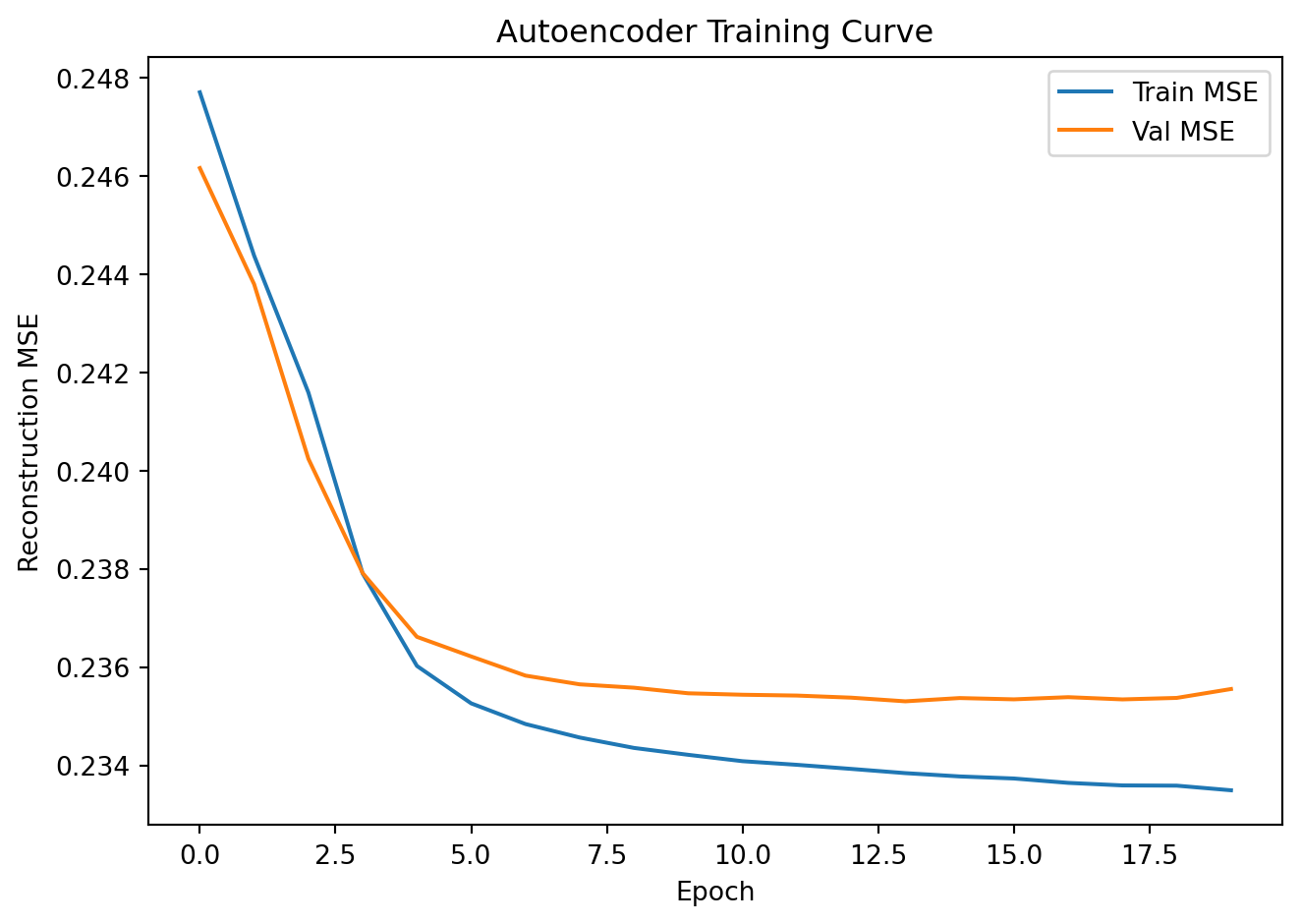
5. Evaluation
Original vs. Reconstructed Images
model.eval()
x_show = torch.stack([val_ds[i][0] for i in range(8)])
with torch.no_grad():
    x_recon, _ = model(x_show)

fig, axes = plt.subplots(2, 8, figsize=(16, 4))
for i in range(8):
    axes[0, i].imshow(x_show[i].squeeze().numpy(), cmap='gray', vmin=0, vmax=1)
    axes[0, i].axis('off')
    axes[1, i].imshow(x_recon[i].squeeze().numpy(), cmap='gray', vmin=0, vmax=1)
    axes[1, i].axis('off')
axes[0, 0].set_ylabel("Original", fontsize=10)
axes[1, 0].set_ylabel("Reconstructed", fontsize=10)
plt.suptitle("Original vs. Reconstructed Ising Configurations")
plt.tight_layout()
plt.show()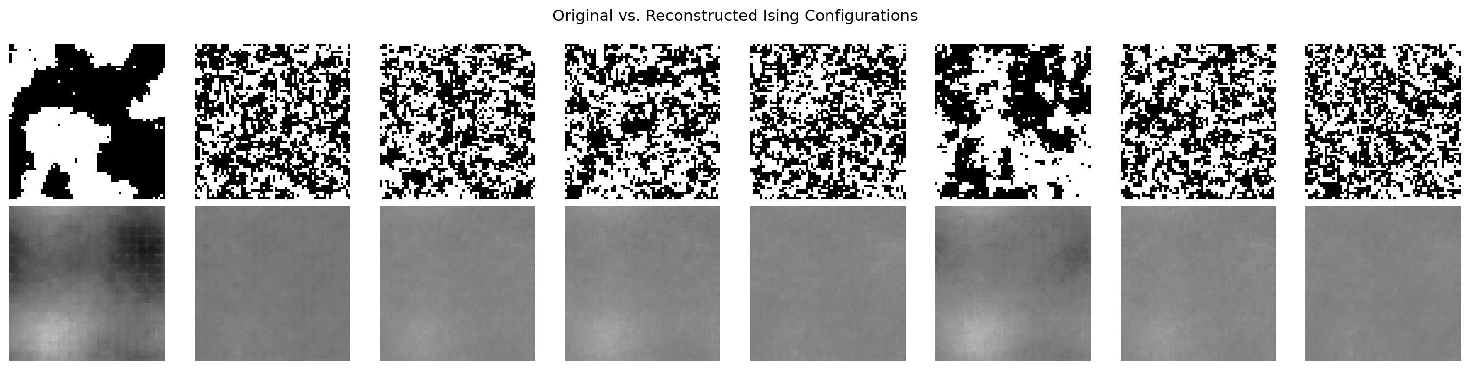
Latent Space Visualization
# Encode all validation samples
all_z, all_labels = [], []
model.eval()
with torch.no_grad():
    for x_batch, y_batch in val_loader:
        _, z = model(x_batch)
        all_z.append(z.numpy())
        all_labels.append(y_batch.numpy())

all_z = np.concatenate(all_z, axis=0)
all_labels = np.concatenate(all_labels, axis=0)

plt.figure(figsize=(7, 6))
for cls, name, color in [(0, "Disordered (T>Tc)", "tab:blue"),
                          (1, "Ordered (T<Tc)", "tab:red")]:
    mask = all_labels == cls
    plt.scatter(all_z[mask, 0], all_z[mask, 1], alpha=0.4, s=10, label=name, color=color)

plt.xlabel("Latent dim 1")
plt.ylabel("Latent dim 2")
plt.title("2D Latent Space — colored by Ising phase")
plt.legend()
plt.tight_layout()
plt.show()

print("Notice how the two phases separate in latent space — the autoencoder")
print("has discovered a representation correlated with the order parameter!")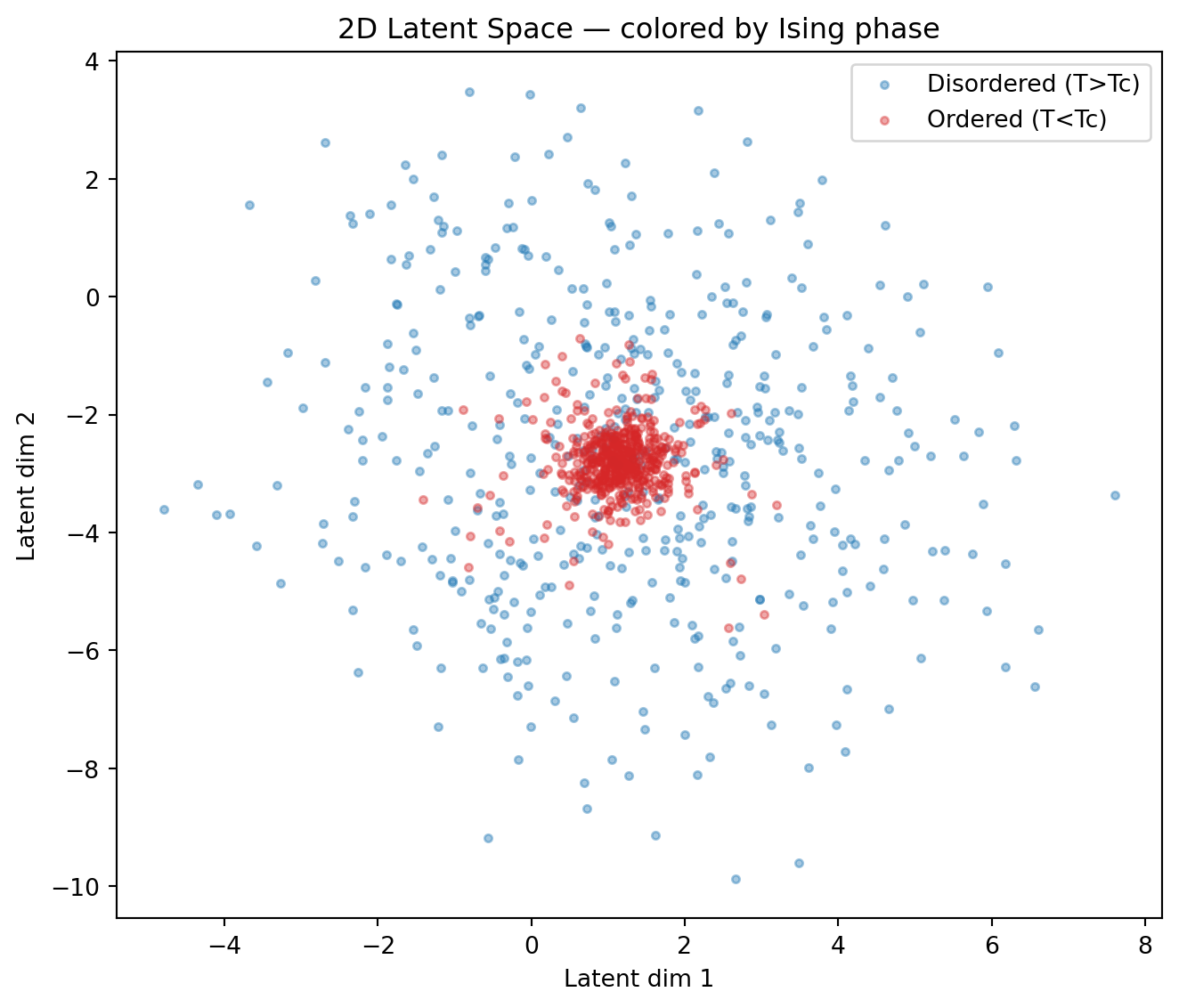
Notice how the two phases separate in latent space — the autoencoder
has discovered a representation correlated with the order parameter!
Exercises
- Try
latent_dim=8. Does reconstruction quality improve? To visualize the 8D space, project to 2D with PCA (from sklearn.decomposition import PCA). Do the phases still separate? - What happens if you feed random Gaussian noise to the decoder? Sample
z = torch.randn(16, 2)and plotmodel.decoder(z). Are the outputs physically meaningful? - Compare the latent space structure to the Ising phase diagram. Can you identify the Curie temperature Tc as a boundary in latent space?