!pip install git+https://github.com/ECLIPSE-Lab/Ai4MatLectures.git "mdsdata>=0.1.5"
!pip install "mace-torch>=0.3.6" "dscribe>=2.1.0"MG Week 6: Local Environments and Universal MLIPs
SOAP fingerprints and MACE-MP-0 single-point + MD on a small bulk-prototype dataset

Learning Objectives
- Compute local atomic-environment fingerprints (SOAP) and visualise how environments cluster by coordination motif rather than by element.
- Run a universal ML interatomic potential (MACE-MP-0) for single-point energy and force evaluation on bulk prototypes across the periodic table.
- Benchmark MACE-MP-0 against a DFT/experimental reference (equilibrium lattice parameter and bulk modulus from an equation-of-state scan).
- Plug the universal MLIP into an ASE NVE molecular-dynamics loop and check energy conservation.
This notebook closes the loop from MG W4/W5 (atomistic simulation as a DFT-accuracy data generator) by replacing the expensive DFT/Hartree-Fock single-point with a near-DFT ML surrogate that runs in milliseconds.
Setup
import time
import numpy as np
import matplotlib.pyplot as plt

from ase import Atoms, units
from ase.build import bulk, make_supercell
from ase.md.velocitydistribution import MaxwellBoltzmannDistribution
from ase.md.verlet import VelocityVerlet

from dscribe.descriptors import SOAP

np.random.seed(0)
Loading the MACE-MP-0 calculator downloads ~50 MB of weights on first use. On Colab this takes a few seconds; on a slow connection it can take a minute. The “small” variant is fine for everything below.
from mace.calculators import mace_mp
mace_calc = mace_mp(model="small", default_dtype="float32", device="cpu")
1. Build a small bulk-prototype dataset
Five elemental / binary prototypes spanning metallic (Cu, Fe, Al), covalent (Si), and ionic (NaCl, MgO) bonding. Each cell is repeated \(2\times 2\times 2\) so SOAP averages and MD have a non-trivial number of atoms.
prototypes = [
    ("Cu",  "fcc",        3.615),
    ("Fe",  "bcc",        2.866),
    ("Al",  "fcc",        4.046),
    ("Si",  "diamond",    5.431),
    ("NaCl","rocksalt",   5.640),
    ("MgO", "rocksalt",   4.212),
]

structures: list[Atoms] = []
labels: list[str] = []
for name, prot, a in prototypes:
    cell = bulk(name, prot, a=a).repeat((2, 2, 2))
    structures.append(cell)
    labels.append(name)
    print(f"{name:>4s}  {prot:>9s}  a₀ = {a:.3f} Å  →  {len(cell):3d} atoms / cell")
Cu fcc a₀ = 3.615 Å → 8 atoms / cell
Fe bcc a₀ = 2.866 Å → 8 atoms / cell
Al fcc a₀ = 4.046 Å → 8 atoms / cell
Si diamond a₀ = 5.431 Å → 16 atoms / cell
NaCl rocksalt a₀ = 5.640 Å → 16 atoms / cell
MgO rocksalt a₀ = 4.212 Å → 16 atoms / cell2. SOAP fingerprints: local environments cluster by coordination
SOAP (Bartók et al. 2013) expands the local atomic density around every atom in a basis of spherical harmonics and radial functions, then takes a rotation-invariant power spectrum. The result is a fixed-length fingerprint per atom that captures the local environment but is invariant to rotation and atom permutation within a species.
species = sorted({s.symbol for atoms in structures for s in atoms})
soap = SOAP(species=species, periodic=True,
            r_cut=4.5, n_max=6, l_max=4, sigma=0.4, sparse=False)
print(f"SOAP fingerprint length per atom: {soap.get_number_of_features()}")
SOAP fingerprint length per atom: 5880Compute per-atom fingerprints, then pool to a single fingerprint per structure by averaging across atoms (this is what most baseline materials ML models do).
per_atom_descs = []
struct_id = []
for i, atoms in enumerate(structures):
    desc = soap.create(atoms)                   # (n_atoms, n_features)
    per_atom_descs.append(desc)
    struct_id.append(np.full(len(atoms), i))

X_atom = np.concatenate(per_atom_descs, axis=0)
ids_atom = np.concatenate(struct_id, axis=0)
print(f"X_atom shape: {X_atom.shape}   (atoms across all structures)")

X_struct = np.stack([d.mean(axis=0) for d in per_atom_descs], axis=0)
print(f"X_struct shape: {X_struct.shape}   (per-structure mean)")
X_atom shape: (72, 5880) (atoms across all structures)
X_struct shape: (6, 5880) (per-structure mean)A 2-D PCA of the per-atom fingerprints visualises the coordination clusters. Atoms with the same coordination motif (FCC 12-fold, BCC 8-fold, diamond 4-fold, rocksalt 6-fold) land in distinct islands, regardless of element — the descriptor is geometric, not chemical.
X_centered = X_atom - X_atom.mean(axis=0, keepdims=True)
_, _, Vt = np.linalg.svd(X_centered, full_matrices=False)
Z = X_centered @ Vt[:2].T

fig, ax = plt.subplots(figsize=(6.5, 5))
colors = plt.cm.tab10(np.linspace(0, 1, len(structures)))
for i, name in enumerate(labels):
    mask = ids_atom == i
    ax.scatter(Z[mask, 0], Z[mask, 1], s=30, alpha=0.7,
               color=colors[i], label=name)
ax.set_xlabel("PC 1"); ax.set_ylabel("PC 2")
ax.set_title("SOAP fingerprints — 2-D PCA, coloured by structure")
ax.legend(loc="best")
plt.tight_layout(); plt.show()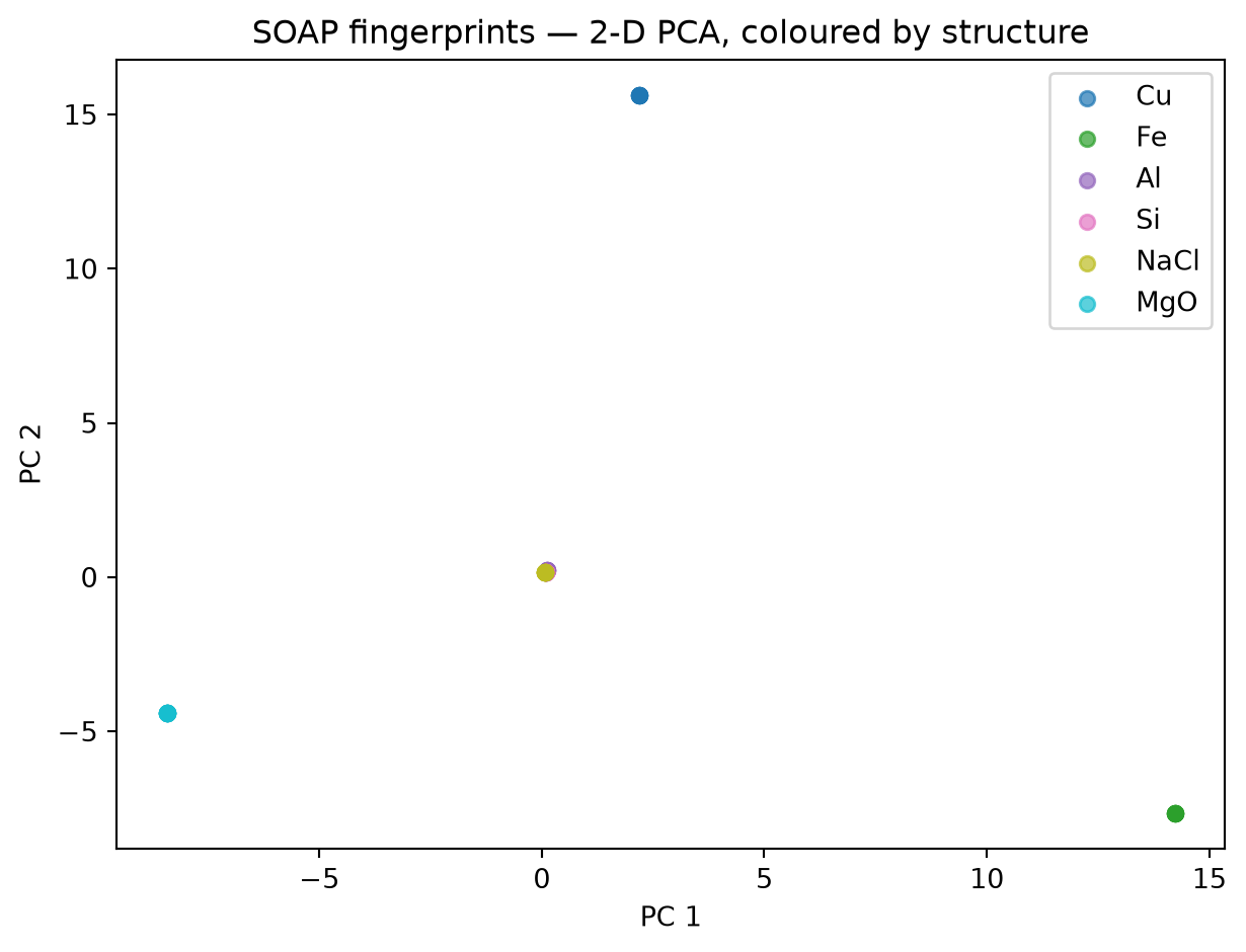
Tip
Read this plot. The metallic FCC and BCC environments separate along PC 1 by coordination number (12 vs 8 nearest neighbours). NaCl and MgO sit close to each other despite being chemically very different — they share the rocksalt 6-fold coordination motif. SOAP sees structure, not chemistry.
3. MACE-MP-0 single-point — energy and forces
MACE-MP-0 (Batatia et al. 2023) is a universal equivariant message-passing potential trained on the Materials Project / Alexandria dataset. A single set of weights covers most of the periodic table at near-DFT accuracy. We attach it as an ASE Calculator and ask for potential energy and forces on each prototype cell.
energies_mace = []
fmax_mace = []
n_atoms = []
times_mace = []
for atoms, name in zip(structures, labels):
    atoms_c = atoms.copy()
    atoms_c.calc = mace_calc
    t0 = time.perf_counter()
    e = atoms_c.get_potential_energy()
    f = atoms_c.get_forces()
    dt = time.perf_counter() - t0
    energies_mace.append(e)
    fmax_mace.append(np.linalg.norm(f, axis=1).max())
    n_atoms.append(len(atoms_c))
    times_mace.append(dt)
    print(f"{name:>5s}  N={len(atoms_c):3d}  E = {e:+9.3f} eV  "
          f"|F|_max = {np.linalg.norm(f, axis=1).max():.3e} eV/Å  "
          f"t = {dt*1e3:7.1f} ms")
Note
Equilibrium bulk cells should have \(|F|_\text{max} \approx 0\) by symmetry — any nonzero value is the MACE-MP-0 force residual on the ideal lattice. Typical magnitudes are \(10^{-3}\,\)eV/Å, well below DFT-convergence thresholds.
4. Equation-of-state benchmark: lattice parameter and bulk modulus
Absolute MACE-MP-0 energies are not directly comparable to DFT cohesive energies — the model uses learned atomic references. The cleanest apples-to-apples benchmark is the equation of state: scan the lattice parameter, fit a parabola, and compare the predicted equilibrium \(a_0\) and bulk modulus \(B_0\) to reference values.
DFT_REFERENCE = {     # PBE / experimental, in (Å, GPa)
    "Cu":  (3.615, 140.0),
    "Fe":  (2.866, 170.0),
    "Al":  (4.046,  76.0),
    "Si":  (5.431,  98.0),
    "NaCl":(5.640,  25.0),
    "MgO": (4.212, 165.0),
}

results = []
for (name, prot, a0_ref), atoms_ref in zip(prototypes, structures):
    scales = np.linspace(0.96, 1.04, 9)
    volumes, energies = [], []
    for s in scales:
        cell = bulk(name, prot, a=a0_ref * s).repeat((2, 2, 2))
        cell.calc = mace_calc
        volumes.append(cell.get_volume() / len(cell))
        energies.append(cell.get_potential_energy() / len(cell))
    volumes = np.array(volumes); energies = np.array(energies)
    # Quadratic fit around the minimum: E(V) ≈ E0 + 0.5 * B/V0 * (V - V0)^2
    p = np.polyfit(volumes, energies, 2)
    V0 = -p[1] / (2 * p[0])
    E0 = np.polyval(p, V0)
    B0_GPa = 2 * p[0] * V0 * 160.21766   # eV/ų → GPa
    a0_mace = (V0 * len(atoms_ref) / np.prod(np.diag(atoms_ref.cell.array) / a0_ref)) ** (1/3)
    a0_ref_, B0_ref = DFT_REFERENCE[name]
    results.append((name, a0_mace, a0_ref_, B0_GPa, B0_ref))
    print(f"{name:>5s}  a₀(MACE) = {a0_mace:6.3f} Å  (ref {a0_ref_:.3f})  "
          f"|  B₀(MACE) = {B0_GPa:6.1f} GPa  (ref {B0_ref:.0f})")
Plot the EOS error so you can see how the universal potential compares to its reference across bonding types.
fig, axes = plt.subplots(1, 2, figsize=(11, 4))
names = [r[0] for r in results]
axes[0].bar(names, [(r[1] - r[2]) / r[2] * 100 for r in results])
axes[0].set_ylabel("Δa₀ / a₀_ref  [%]")
axes[0].axhline(0, color="k", lw=0.5)
axes[0].set_title("Lattice-parameter error vs reference")
axes[1].bar(names, [(r[3] - r[4]) / r[4] * 100 for r in results])
axes[1].set_ylabel("ΔB₀ / B₀_ref  [%]")
axes[1].axhline(0, color="k", lw=0.5)
axes[1].set_title("Bulk-modulus error vs reference")
plt.tight_layout(); plt.show()
Tip
What to look for. Lattice parameters are usually within ~1% — that is the accuracy bar MACE-MP-0 was trained against. Bulk moduli can deviate by 10–20%, especially for ionic systems where polarisation matters. Universal MLIPs are near-DFT, not exact-DFT; they shine on geometry and break harder on linear-response properties.
5. Plug MACE-MP-0 into an MD loop
A universal MLIP only becomes useful when you can run dynamics with it. Here we run a short NVE Velocity-Verlet trajectory on bulk Cu at 300 K and check energy conservation — the diagnostic test for any new potential.
md_atoms = bulk("Cu", "fcc", a=3.615).repeat((3, 3, 3))   # 108 atoms
md_atoms.calc = mace_calc
MaxwellBoltzmannDistribution(md_atoms, temperature_K=300, rng=np.random.default_rng(0))

dyn = VelocityVerlet(md_atoms, timestep=1.0 * units.fs)
n_steps = 200          # 0.2 ps
hist_E_kin, hist_E_pot, hist_T = [], [], []
t0 = time.perf_counter()
for step in range(n_steps):
    dyn.run(1)
    E_kin = md_atoms.get_kinetic_energy() / len(md_atoms)
    E_pot = md_atoms.get_potential_energy() / len(md_atoms)
    T = md_atoms.get_temperature()
    hist_E_kin.append(E_kin); hist_E_pot.append(E_pot); hist_T.append(T)
print(f"MD: {n_steps} steps on N={len(md_atoms)} atoms  "
      f"→  {(time.perf_counter() - t0):.1f} s total, "
      f"{(time.perf_counter() - t0) / n_steps * 1000:.0f} ms / step")
hist_E_kin = np.array(hist_E_kin); hist_E_pot = np.array(hist_E_pot)
E_tot = hist_E_kin + hist_E_pot
t_ps = np.arange(n_steps) * 1e-3
fig, axes = plt.subplots(1, 2, figsize=(11, 4))
axes[0].plot(t_ps, hist_E_kin, label="E_kin")
axes[0].plot(t_ps, hist_E_pot - hist_E_pot[0] + hist_E_kin[0], label="E_pot (shifted)")
axes[0].plot(t_ps, E_tot - E_tot[0] + 2 * hist_E_kin[0], "k--", label="E_tot (shifted)")
axes[0].set_xlabel("time [ps]"); axes[0].set_ylabel("Energy / atom [eV]")
axes[0].legend(); axes[0].set_title("Energy components")
axes[1].plot(t_ps, hist_T)
axes[1].set_xlabel("time [ps]"); axes[1].set_ylabel("instantaneous T [K]")
axes[1].set_title("Equilibration around 300 K")
plt.tight_layout(); plt.show()
print(f"Total-energy drift: {(E_tot[-1] - E_tot[0]) * 1e3:.3f} meV/atom over {t_ps[-1]:.2f} ps")
Note
A well-behaved MLIP-MD run keeps the total energy drift below ~1 meV/atom over 1 ps for a 1 fs timestep. Larger drifts indicate either too coarse a timestep or pathological extrapolation outside the training distribution. This is the same conservation test you would apply to any new force field.
Exercises
Stretch the periodic table. Add three more prototypes to the dataset — e.g., hcp Ti, diamond C, perovskite SrTiO₃ — and rerun sections 3–4. For which of these does MACE-MP-0 deviate most from its reference? Hypothesise why before looking up the answer.
Out-of-distribution probe. Take a Cu cell, randomly displace every atom by a uniform 0.3 Å in each Cartesian direction, and ask MACE-MP-0 for the energy. Now do the same for 0.6 Å and 1.0 Å. At what displacement does the force magnitude exceed \(1\,\)eV/Å — a rough OOD warning sign?
Replace the back-end. Swap
mace_mp(model="small")formace_mp(model="large")(heavier, more accurate) and rerun section 4. How much does the bulk-modulus error drop, and what is the runtime cost?Stretch — alternative universal MLIPs. If you have the bandwidth, install
orb-modelsormattersimand reproduce section 3 with the alternative back-end. Compare the per-atom energy ordering of the prototypes across the three potentials and discuss which features of the chemistry each model gets right.