MG Week 8: Generalization and Learning Curves

Train/val/test protocol and decision boundaries on NanoindentationDataset

Open In Colab

Learning Objectives

• Apply a rigorous train/val/test protocol to evaluate generalization
• Generate learning curves to understand sample efficiency
• Visualize 2D decision boundaries for a low-dimensional classifier

Setup

!pip install git+https://github.com/ECLIPSE-Lab/Ai4MatLectures.git "mdsdata>=0.1.5"

import torch
import torch.nn as nn
from torch.utils.data import DataLoader, random_split, Subset
from ai4mat.datasets import NanoindentationDataset
import matplotlib.pyplot as plt
import numpy as np

1. Load the Data

dataset = NanoindentationDataset()
print(f"Dataset size: {len(dataset)}")
x0, y0 = dataset[0]
print(f"Sample x shape: {x0.shape}  (features: E [GPa], H [GPa])")
print(f"Sample y: {y0}  (material class, long)")

X_all = torch.stack([dataset[i][0] for i in range(len(dataset))]).numpy()
y_all = torch.tensor([dataset[i][1] for i in range(len(dataset))]).numpy()

n_classes = len(np.unique(y_all))
print(f"\nClasses: {np.unique(y_all).tolist()}")
print(f"Class counts: {dict(zip(*np.unique(y_all, return_counts=True)))}")

Dataset size: 938
Sample x shape: torch.Size([2])  (features: E [GPa], H [GPa])
Sample y: 0  (material class, long)

Classes: [0, 1, 2, 3]
Class counts: {0: 30, 1: 513, 2: 364, 3: 31}

colors = ['tab:blue', 'tab:orange', 'tab:green', 'tab:red']
plt.figure(figsize=(7, 5))
for cls in range(n_classes):
    mask = y_all == cls
    plt.scatter(X_all[mask, 0], X_all[mask, 1], alpha=0.6, s=20,
                color=colors[cls], label=f"Class {cls}")
plt.xlabel("Young's modulus E (GPa)")
plt.ylabel("Hardness H (GPa)")
plt.title("Nanoindentation dataset — ground truth labels")
plt.legend(); plt.tight_layout(); plt.show()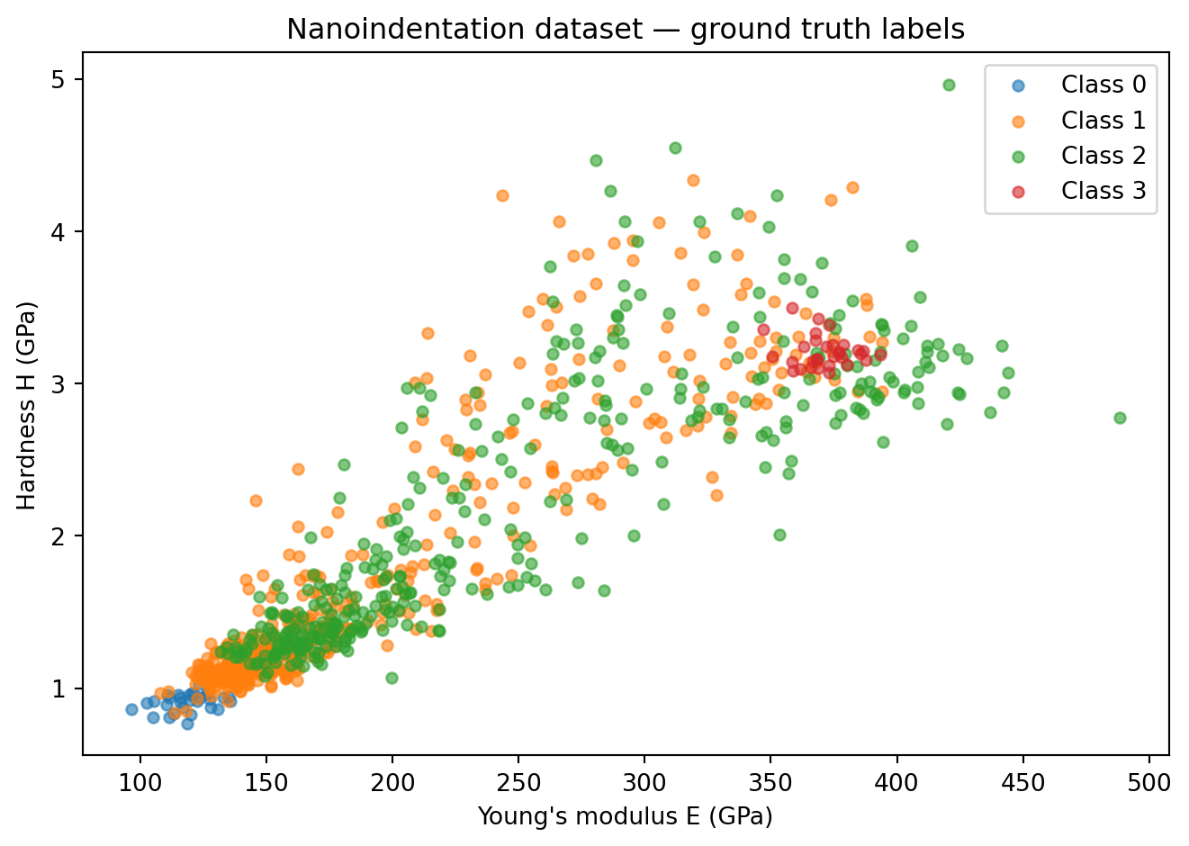

2. Train / Val / Test Split (80 / 10 / 10)

n = len(dataset)
n_train = int(0.8 * n)
n_val   = int(0.1 * n)
n_test  = n - n_train - n_val

torch.manual_seed(42)
train_ds, val_ds, test_ds = random_split(dataset, [n_train, n_val, n_test])

train_loader = DataLoader(train_ds, batch_size=64, shuffle=True)
val_loader   = DataLoader(val_ds,   batch_size=64, shuffle=False)
test_loader  = DataLoader(test_ds,  batch_size=64, shuffle=False)
print(f"Train: {n_train} | Val: {n_val} | Test: {n_test}")

Train: 750 | Val: 93 | Test: 95

3. Define the Model

model = nn.Sequential(
    nn.Linear(2, 32), nn.ReLU(),
    nn.Linear(32, 4)
)
print(model)
print(f"Parameters: {sum(p.numel() for p in model.parameters())}")

Sequential(
  (0): Linear(in_features=2, out_features=32, bias=True)
  (1): ReLU()
  (2): Linear(in_features=32, out_features=4, bias=True)
)
Parameters: 228

4. Training Loop

criterion = nn.CrossEntropyLoss()
optimizer = torch.optim.Adam(model.parameters(), lr=1e-3)

train_accs, val_accs = [], []

for epoch in range(100):
    model.train()
    ep_acc = 0.0
    for x_batch, y_batch in train_loader:
        optimizer.zero_grad()
        logits = model(x_batch)
        loss = criterion(logits, y_batch)
        loss.backward()
        optimizer.step()
        ep_acc += (logits.argmax(1) == y_batch).float().sum().item()
    train_accs.append(ep_acc / n_train)

    model.eval()
    v_acc = 0.0
    with torch.no_grad():
        for x_batch, y_batch in val_loader:
            logits = model(x_batch)
            v_acc += (logits.argmax(1) == y_batch).float().sum().item()
    val_accs.append(v_acc / n_val)

plt.plot(train_accs, label='Train'); plt.plot(val_accs, label='Val')
plt.xlabel("Epoch"); plt.ylabel("Accuracy"); plt.legend()
plt.title("Training Curve"); plt.tight_layout(); plt.show()

# Final test accuracy (only inspect once!)
model.eval()
test_acc = 0.0
with torch.no_grad():
    for x_batch, y_batch in test_loader:
        logits = model(x_batch)
        test_acc += (logits.argmax(1) == y_batch).float().sum().item()
print(f"Test accuracy: {test_acc / n_test:.3f}")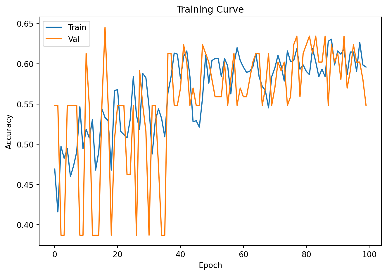

Test accuracy: 0.526

5. Decision Boundary Visualization

The 2D input space makes it possible to visualize the classifier boundary directly.

# Build a fine grid over the feature space
x_min, x_max = X_all[:, 0].min() - 1, X_all[:, 0].max() + 1
y_min, y_max = X_all[:, 1].min() - 0.5, X_all[:, 1].max() + 0.5
xx, yy = np.meshgrid(np.linspace(x_min, x_max, 300),
                     np.linspace(y_min, y_max, 300))
grid = torch.tensor(np.c_[xx.ravel(), yy.ravel()], dtype=torch.float32)

model.eval()
with torch.no_grad():
    grid_preds = model(grid).argmax(dim=1).numpy()

plt.figure(figsize=(8, 6))
plt.contourf(xx, yy, grid_preds.reshape(xx.shape), alpha=0.3,
             levels=[-0.5, 0.5, 1.5, 2.5, 3.5], colors=colors)
for cls in range(n_classes):
    mask = y_all == cls
    plt.scatter(X_all[mask, 0], X_all[mask, 1], s=20, alpha=0.7,
                color=colors[cls], label=f"Class {cls}")
plt.xlabel("E (GPa)"); plt.ylabel("H (GPa)")
plt.title("Decision Boundary (shaded regions = predicted class)")
plt.legend(); plt.tight_layout(); plt.show()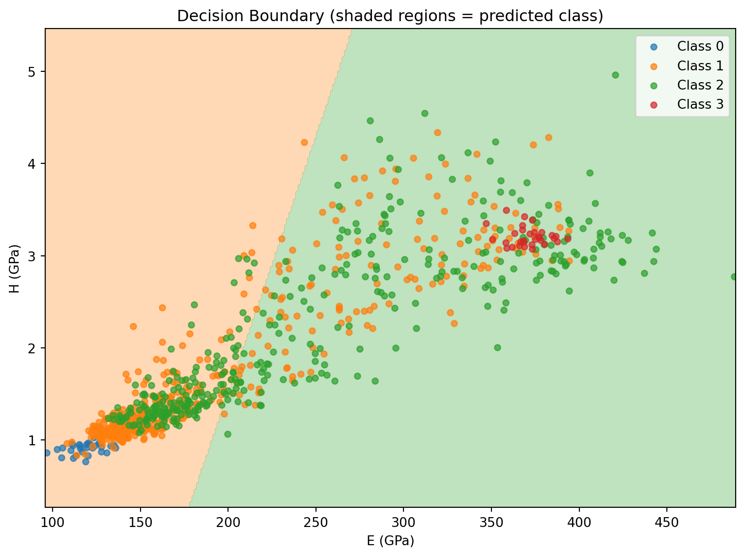

6. Learning Curve (Sample Efficiency)

How much training data do we really need?

fractions = [0.10, 0.20, 0.30, 0.40, 0.50, 0.60, 0.70, 0.80]
test_accs_by_size = []

all_train_indices = list(train_ds.indices)
np.random.seed(42)

for frac in fractions:
    n_sub = max(10, int(frac * n_train))
    sub_idx = np.random.choice(all_train_indices, size=n_sub, replace=False).tolist()
    sub_ds = Subset(dataset, sub_idx)
    sub_loader = DataLoader(sub_ds, batch_size=32, shuffle=True)

    m = nn.Sequential(nn.Linear(2, 32), nn.ReLU(), nn.Linear(32, 4))
    opt = torch.optim.Adam(m.parameters(), lr=1e-3)
    torch.manual_seed(0)
    for _ in range(100):
        m.train()
        for xb, yb in sub_loader:
            opt.zero_grad(); criterion(m(xb), yb).backward(); opt.step()

    m.eval()
    ta = 0.0
    with torch.no_grad():
        for xb, yb in test_loader:
            ta += (m(xb).argmax(1) == yb).float().sum().item()
    test_accs_by_size.append(ta / n_test)
    print(f"  {int(frac*100):3d}% training ({n_sub:4d} samples) → test acc: {ta/n_test:.3f}")

plt.figure(figsize=(7, 4))
plt.plot([int(f * n_train) for f in fractions], test_accs_by_size, 'o-')
plt.xlabel("Number of training samples")
plt.ylabel("Test accuracy")
plt.title("Learning Curve")
plt.grid(True); plt.tight_layout(); plt.show()

   10% training (  75 samples) → test acc: 0.547
   20% training ( 150 samples) → test acc: 0.568
   30% training ( 225 samples) → test acc: 0.558
   40% training ( 300 samples) → test acc: 0.558
   50% training ( 375 samples) → test acc: 0.547
   60% training ( 450 samples) → test acc: 0.568
   70% training ( 525 samples) → test acc: 0.558
   80% training ( 600 samples) → test acc: 0.547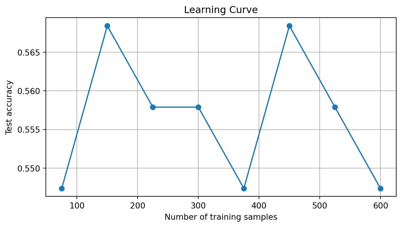

Exercises

1. From the learning curve, what minimum number of training samples achieves >90% test accuracy?
2. Compare the MLP decision boundary to k-NN: from sklearn.neighbors import KNeighborsClassifier. Fit k-NN with k=5 on the same training data and visualize its boundary — is it smoother or rougher than the MLP?
3. The test set should be held out until the very end. Why is it wrong to use test accuracy to tune hyperparameters (like hidden layer size)? Redesign the experiment to properly use only train and val for model selection.