!pip install git+https://github.com/ECLIPSE-Lab/Ai4MatLectures.git "mdsdata>=0.1.5"MG Week 11: Latent Space and Phase Transitions
Autoencoder representations of Ising spin configurations
![]()
Learning Objectives
- Understand latent spaces as learned low-dimensional representations
- Connect the 2D latent space structure to physical phase behavior
- Recognize that autoencoders can discover order parameters without supervision
Setup
import torch
import torch.nn as nn
from torch.utils.data import DataLoader, random_split
from ai4mat.datasets import IsingDataset
import matplotlib.pyplot as plt
import numpy as np
1. Load the Data
dataset = IsingDataset(size='light')
print(f"Dataset size: {len(dataset)}")
x0, y0 = dataset[0]
print(f"Sample x shape: {x0.shape}  (1, 16, 16)")
print(f"Sample y: {y0}  (0 = T > Tc disordered, 1 = T < Tc ordered)")

y_all_check = torch.tensor([dataset[i][1].item() for i in range(len(dataset))])
print(f"Class balance: {(y_all_check == 0).sum().item()} disordered, {(y_all_check == 1).sum().item()} ordered")
Dataset size: 5000
Sample x shape: torch.Size([1, 16, 16]) (1, 16, 16)
Sample y: 1 (0 = T > Tc disordered, 1 = T < Tc ordered)
Class balance: 2507 disordered, 2493 orderedfig, axes = plt.subplots(2, 5, figsize=(14, 6))
for i, ax in enumerate(axes.flat):
idx = i * (len(dataset) // 10)
img = dataset[idx][0].squeeze().numpy()
label = dataset[idx][1].item()
ax.imshow(img, cmap='gray', vmin=0, vmax=1)
ax.set_title(f"{'Ordered' if label==1 else 'Disordered'}", fontsize=8)
ax.axis('off')
plt.suptitle("Ising spin configurations (16×16)")
plt.tight_layout()
plt.show()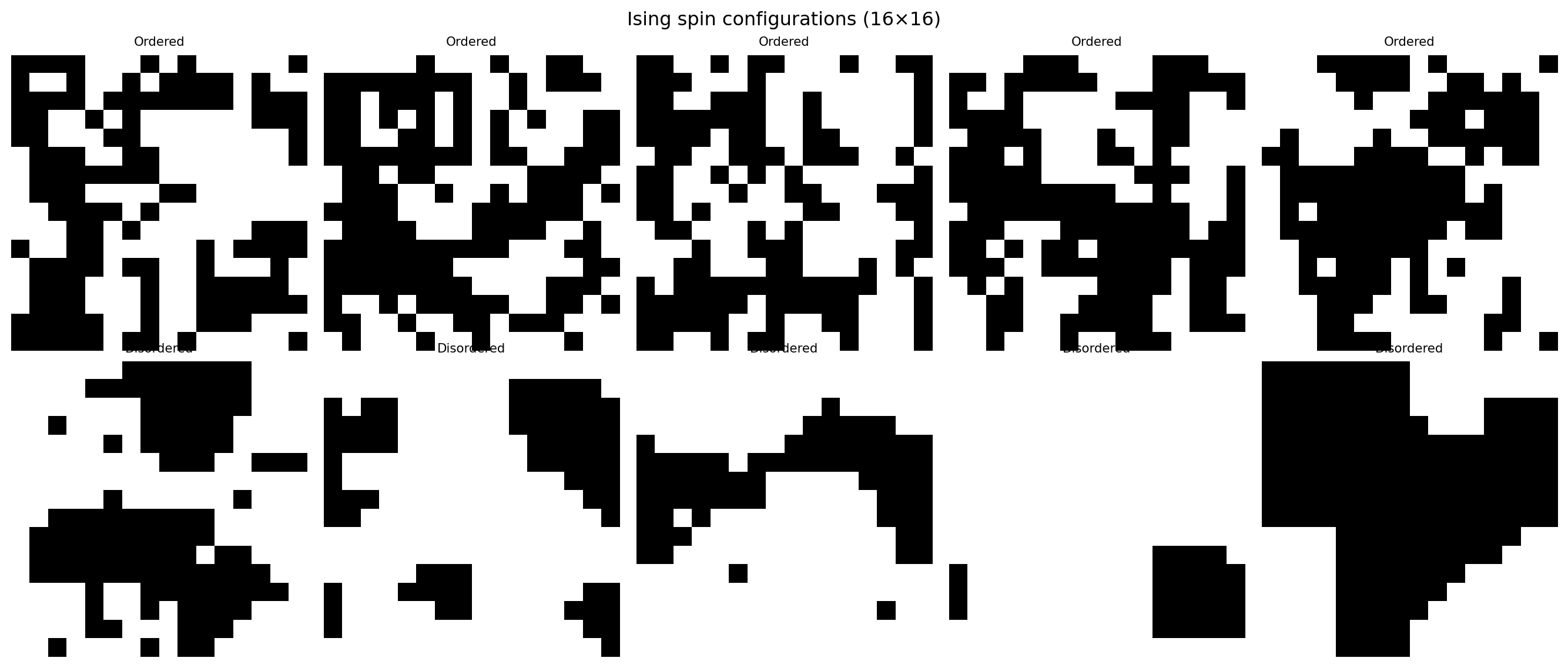
2. Train/Val Split
n_train = int(0.8 * len(dataset))
n_val = len(dataset) - n_train
train_ds, val_ds = random_split(dataset, [n_train, n_val])

train_loader = DataLoader(train_ds, batch_size=64, shuffle=True)
val_loader   = DataLoader(val_ds,   batch_size=64, shuffle=False)
print(f"Train: {n_train} | Val: {n_val}")
Train: 4000 | Val: 10003. Define the Autoencoder
The autoencoder is trained WITHOUT labels — it must reconstruct input images from a 2D bottleneck. The latent space emerges from the structure in the data.
class ConvAutoencoder(nn.Module):
    def __init__(self, latent_dim=2):
        super().__init__()
        self.encoder = nn.Sequential(
            nn.Conv2d(1, 16, 3, stride=2, padding=1),   # 8x8
            nn.ReLU(),
            nn.Conv2d(16, 32, 3, stride=2, padding=1),  # 4x4
            nn.ReLU(),
            nn.Flatten(),
            nn.Linear(32 * 4 * 4, latent_dim)
        )
        self.decoder = nn.Sequential(
            nn.Linear(latent_dim, 32 * 4 * 4),
            nn.ReLU(),
            nn.Unflatten(1, (32, 4, 4)),
            nn.ConvTranspose2d(32, 16, 3, stride=2, padding=1, output_padding=1),  # 8x8
            nn.ReLU(),
            nn.ConvTranspose2d(16, 1, 3, stride=2, padding=1, output_padding=1),   # 16x16
            nn.Sigmoid()
        )

    def forward(self, x):
        z = self.encoder(x)
        return self.decoder(z), z

model = ConvAutoencoder(latent_dim=2)
n_params = sum(p.numel() for p in model.parameters())
print(f"Autoencoder parameters: {n_params:,}")

# Verify shapes
x_test = torch.zeros(4, 1, 16, 16)
x_recon, z = model(x_test)
print(f"Input:   {x_test.shape}")
print(f"Latent:  {z.shape}")
print(f"Output:  {x_recon.shape}")
Autoencoder parameters: 12,131
Input: torch.Size([4, 1, 16, 16])
Latent: torch.Size([4, 2])
Output: torch.Size([4, 1, 16, 16])4. Training Loop
criterion = nn.MSELoss()
optimizer = torch.optim.Adam(model.parameters(), lr=1e-3)

train_losses, val_losses = [], []

for epoch in range(20):
    model.train()
    ep_loss = 0.0
    for x_batch, _ in train_loader:    # No labels used!
        optimizer.zero_grad()
        x_recon, _ = model(x_batch)
        loss = criterion(x_recon, x_batch)
        loss.backward()
        optimizer.step()
        ep_loss += loss.item() * len(x_batch)
    train_losses.append(ep_loss / n_train)

    model.eval()
    v_loss = 0.0
    with torch.no_grad():
        for x_batch, _ in val_loader:
            x_recon, _ = model(x_batch)
            v_loss += criterion(x_recon, x_batch).item() * len(x_batch)
    val_losses.append(v_loss / n_val)

    if (epoch + 1) % 5 == 0:
        print(f"Epoch {epoch+1:3d} | Train MSE: {train_losses[-1]:.4f} | Val MSE: {val_losses[-1]:.4f}")

plt.plot(train_losses, label='Train MSE')
plt.plot(val_losses,   label='Val MSE')
plt.xlabel("Epoch"); plt.ylabel("Reconstruction MSE")
plt.title("Autoencoder Training"); plt.legend()
plt.tight_layout(); plt.show()
Epoch 5 | Train MSE: 0.1971 | Val MSE: 0.1973
Epoch 10 | Train MSE: 0.1952 | Val MSE: 0.1963
Epoch 15 | Train MSE: 0.1944 | Val MSE: 0.1963
Epoch 20 | Train MSE: 0.1941 | Val MSE: 0.1962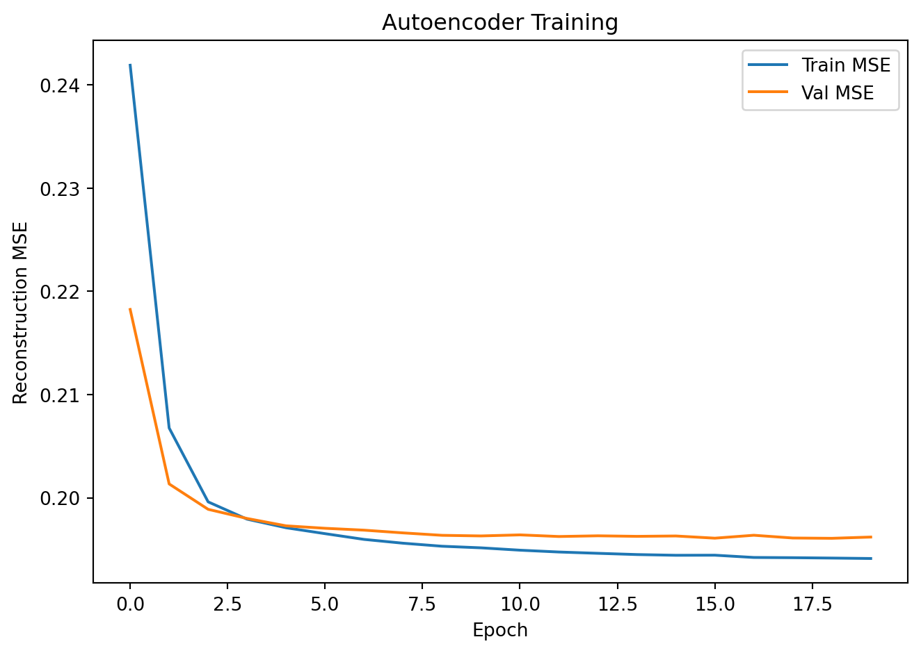
5. Latent Space Visualization
# Encode all data
all_z, all_labels = [], []
model.eval()
full_loader = DataLoader(dataset, batch_size=64, shuffle=False)
with torch.no_grad():
    for x_batch, y_batch in full_loader:
        _, z = model(x_batch)
        all_z.append(z.numpy())
        all_labels.append(y_batch.numpy())

all_z = np.concatenate(all_z, axis=0)
all_labels = np.concatenate(all_labels, axis=0)

fig, ax = plt.subplots(figsize=(7, 6))
for cls, name, color in [(0, "Disordered (T > Tc)", "tab:blue"),
                          (1, "Ordered   (T < Tc)", "tab:red")]:
    mask = all_labels == cls
    ax.scatter(all_z[mask, 0], all_z[mask, 1], alpha=0.35, s=12,
               color=color, label=name)

ax.set_xlabel("Latent dim 1")
ax.set_ylabel("Latent dim 2")
ax.set_title("2D Latent Space — colored by Ising phase")
ax.legend()
plt.tight_layout()
plt.show()

print("Key observation: the AE was trained with NO phase labels.")
print("Yet the latent space has discovered a representation that separates")
print("the two phases — essentially learning the magnetic order parameter!")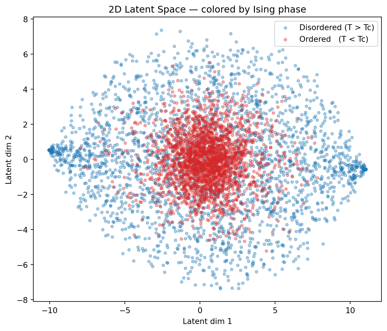
Key observation: the AE was trained with NO phase labels.
Yet the latent space has discovered a representation that separates
the two phases — essentially learning the magnetic order parameter!
# Reconstruct some images
fig, axes = plt.subplots(2, 8, figsize=(16, 4))
x_show = torch.stack([val_ds[i][0] for i in range(8)])
with torch.no_grad():
x_recon, _ = model(x_show)
for i in range(8):
axes[0, i].imshow(x_show[i].squeeze().numpy(), cmap='gray', vmin=0, vmax=1)
axes[1, i].imshow(x_recon[i].squeeze().numpy(), cmap='gray', vmin=0, vmax=1)
axes[0, i].axis('off'); axes[1, i].axis('off')
axes[0, 0].set_ylabel("Original", fontsize=9)
axes[1, 0].set_ylabel("Reconstructed", fontsize=9)
plt.suptitle("Original vs. Reconstructed Ising Configurations")
plt.tight_layout(); plt.show()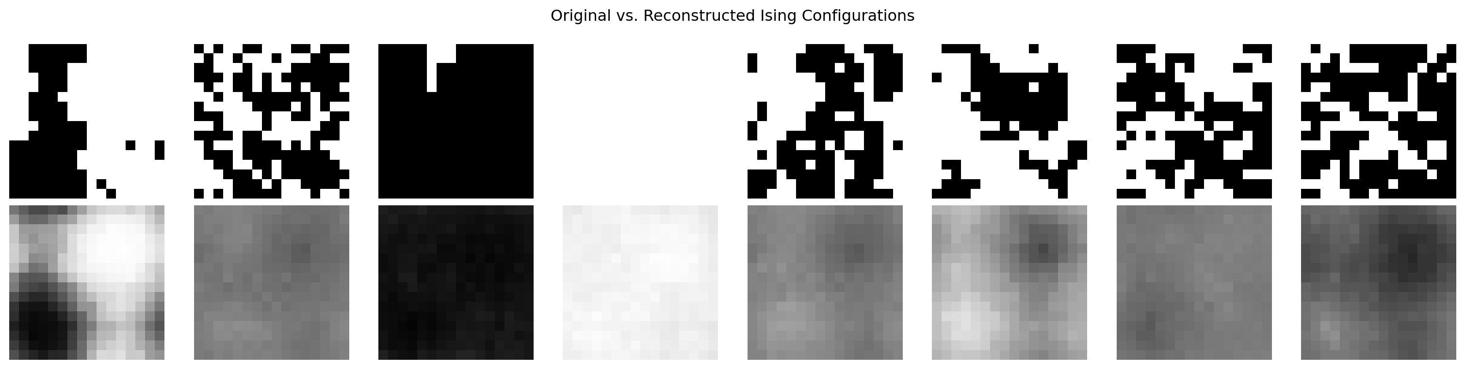
Physics Connection
print("The Ising model undergoes a phase transition at the Curie temperature Tc.")
print()
print("Below Tc (label=1): spins align → ferromagnetic order → high magnetization")
print("Above Tc (label=0): spins random → paramagnetic → zero net magnetization")
print()
print("The order parameter for this transition is the magnetization M = <σ>.")
print()
print("Our autoencoder — trained purely to reconstruct images — has implicitly")
print("learned a 2D representation where the two phases are spatially separated.")
print("This is a remarkable example of unsupervised discovery of physical structure!")
The Ising model undergoes a phase transition at the Curie temperature Tc.
Below Tc (label=1): spins align → ferromagnetic order → high magnetization
Above Tc (label=0): spins random → paramagnetic → zero net magnetization
The order parameter for this transition is the magnetization M = <σ>.
Our autoencoder — trained purely to reconstruct images — has implicitly
learned a 2D representation where the two phases are spatially separated.
This is a remarkable example of unsupervised discovery of physical structure!Exercises
- Try
latent_dim=1. Can a single latent coordinate still separate the two phases? Plot the 1D latent values colored by label. - Try
latent_dim=4. Visualize the 4D latent space by projecting to 2D with PCA:from sklearn.decomposition import PCA; z_2d = PCA(2).fit_transform(all_z). Does the phase separation persist? - Try latent space interpolation: pick two latent codes from opposite phases, interpolate 10 steps linearly, decode each, and plot. What does the reconstructed image look like in between the two phases?