!pip install git+https://github.com/ECLIPSE-Lab/Ai4MatLectures.git "mdsdata>=0.1.5"MLPC Week 4: Linear Baseline for Digit Classification
Logistic regression on DigitsDataset before going deep
![]()
Learning Objectives
- Establish a linear baseline before building more complex models
- Understand why linear models struggle with raw pixel features
- Interpret the learned weight matrix as a set of class templates
Setup
import torch
import torch.nn as nn
from torch.utils.data import DataLoader, random_split
from ai4mat.datasets import DigitsDataset
import matplotlib.pyplot as plt
import numpy as np
1. Load the Data
dataset = DigitsDataset()
print(f"Dataset size: {len(dataset)}")
x0, y0 = dataset[0]
print(f"Sample x shape: {x0.shape}, dtype: {x0.dtype}  (flattened 8×8 image)")
print(f"Sample y: {y0}")

X_all = torch.stack([dataset[i][0] for i in range(len(dataset))])
y_all = torch.tensor([dataset[i][1] for i in range(len(dataset))])
print(f"\nAll classes: {torch.unique(y_all).tolist()}")
Dataset size: 5620
Sample x shape: torch.Size([64]), dtype: torch.float32 (flattened 8×8 image)
Sample y: 0
All classes: [0, 1, 2, 3, 4, 5, 6, 7, 8, 9]# Show sample images
fig, axes = plt.subplots(2, 10, figsize=(16, 4))
for digit in range(10):
idxs = (y_all == digit).nonzero(as_tuple=True)[0][:2]
for row, idx in enumerate(idxs):
axes[row, digit].imshow(X_all[idx].reshape(8, 8).numpy(), cmap='gray_r')
axes[row, digit].set_title(str(digit), fontsize=9)
axes[row, digit].axis('off')
plt.suptitle("Two examples per digit class")
plt.tight_layout()
plt.show()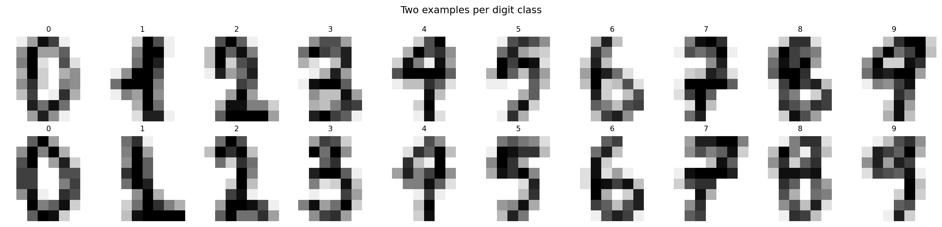
2. Train/Val Split
n_train = int(0.8 * len(dataset))
n_val = len(dataset) - n_train
train_ds, val_ds = random_split(dataset, [n_train, n_val])

train_loader = DataLoader(train_ds, batch_size=64, shuffle=True)
val_loader   = DataLoader(val_ds,   batch_size=64, shuffle=False)
print(f"Train: {n_train} | Val: {n_val}")
Train: 4496 | Val: 11243. Define the Model — Logistic Regression
Research question: What is the best accuracy a linear model can achieve on raw pixel features?
# Logistic regression = single linear layer with CrossEntropyLoss
# (no hidden layers, no nonlinearity)
model = nn.Linear(64, 10)
print(model)
print(f"Parameters: {sum(p.numel() for p in model.parameters()):,}")
print(f"Input:  64 pixel values  →  Output: 10 class logits")
Linear(in_features=64, out_features=10, bias=True)
Parameters: 650
Input: 64 pixel values → Output: 10 class logits4. Training Loop
criterion = nn.CrossEntropyLoss()
optimizer = torch.optim.Adam(model.parameters(), lr=1e-3)

train_losses, val_losses = [], []
train_accs, val_accs = [], []

def accuracy(logits, labels):
    return (logits.argmax(dim=1) == labels).float().mean().item()

for epoch in range(50):
    model.train()
    ep_loss, ep_acc = 0.0, 0.0
    for x_batch, y_batch in train_loader:
        optimizer.zero_grad()
        logits = model(x_batch)
        loss = criterion(logits, y_batch)
        loss.backward()
        optimizer.step()
        ep_loss += loss.item() * len(x_batch)
        ep_acc  += accuracy(logits, y_batch) * len(x_batch)
    train_losses.append(ep_loss / n_train)
    train_accs.append(ep_acc / n_train)

    model.eval()
    v_loss, v_acc = 0.0, 0.0
    with torch.no_grad():
        for x_batch, y_batch in val_loader:
            logits = model(x_batch)
            v_loss += criterion(logits, y_batch).item() * len(x_batch)
            v_acc  += accuracy(logits, y_batch) * len(x_batch)
    val_losses.append(v_loss / n_val)
    val_accs.append(v_acc / n_val)

fig, axes = plt.subplots(1, 2, figsize=(12, 4))
axes[0].plot(train_losses, label='Train'); axes[0].plot(val_losses, label='Val')
axes[0].set_xlabel("Epoch"); axes[0].set_ylabel("Loss"); axes[0].legend()
axes[0].set_title("Loss")
axes[1].plot(train_accs, label='Train'); axes[1].plot(val_accs, label='Val')
axes[1].set_xlabel("Epoch"); axes[1].set_ylabel("Accuracy"); axes[1].legend()
axes[1].set_title("Accuracy")
plt.tight_layout(); plt.show()
print(f"Final val accuracy (linear model): {val_accs[-1]:.3f}")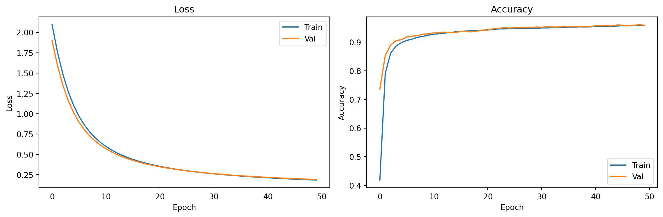
Final val accuracy (linear model): 0.9595. Evaluation
# Visualize the weight matrix as class templates
# Each column of W is a 64-dim vector — reshape to 8x8 image
W = model.weight.data.numpy()  # shape: (10, 64)

fig, axes = plt.subplots(1, 10, figsize=(16, 2))
for digit in range(10):
    template = W[digit].reshape(8, 8)
    vmax = np.abs(template).max()
    axes[digit].imshow(template, cmap='RdBu_r', vmin=-vmax, vmax=vmax)
    axes[digit].set_title(str(digit))
    axes[digit].axis('off')
plt.suptitle("Learned weight templates (red=positive, blue=negative)")
plt.tight_layout()
plt.show()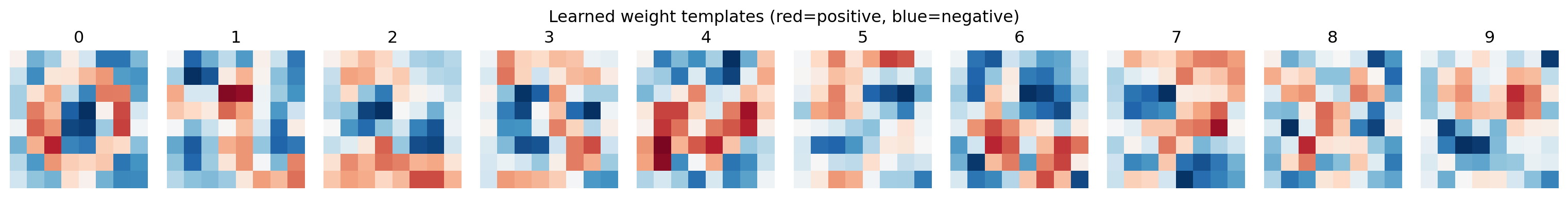
# Find which digits are most confused
model.eval()
conf = torch.zeros(10, 10, dtype=torch.long)
with torch.no_grad():
    for x_batch, y_batch in val_loader:
        preds = model(x_batch).argmax(dim=1)
        for t, p in zip(y_batch, preds):
            conf[t.item(), p.item()] += 1

# Most confused pairs
errors = []
for i in range(10):
    for j in range(10):
        if i != j and conf[i, j] > 0:
            errors.append((conf[i, j].item(), i, j))
errors.sort(reverse=True)
print("Top confusion pairs (true → predicted, count):")
for count, true, pred in errors[:5]:
    print(f"  {true} → {pred}: {count} errors")
Top confusion pairs (true → predicted, count):
1 → 8: 6 errors
9 → 5: 4 errors
5 → 9: 4 errors
4 → 9: 4 errors
8 → 1: 3 errorsExercises
- Add one hidden layer:
nn.Sequential(nn.Linear(64, 32), nn.ReLU(), nn.Linear(32, 10)). By how many percentage points does val accuracy increase? - The weight matrix
model.weighthas shape (10, 64). Plot each row as an 8×8 image. Do they look like digit templates? What does this tell you about what a linear classifier has learned? - Examine the confusion matrix. Which two digits does the linear model confuse most often? Why might those be especially hard?