!pip install git+https://github.com/ECLIPSE-Lab/Ai4MatLectures.git "pymatgen>=2024.3" "matminer>=0.9"MLPC Week 5: Clustering thermoelectric materials (ESTM)
PCA + K-means on element-fraction and Magpie features

Learning Objectives
- Apply K-means to a tabular materials dataset with quantitative property targets.
- Understand how featurization choice (raw fractions vs Magpie physics-aware descriptors) changes cluster geometry.
- Use elbow + silhouette together to motivate a cluster count.
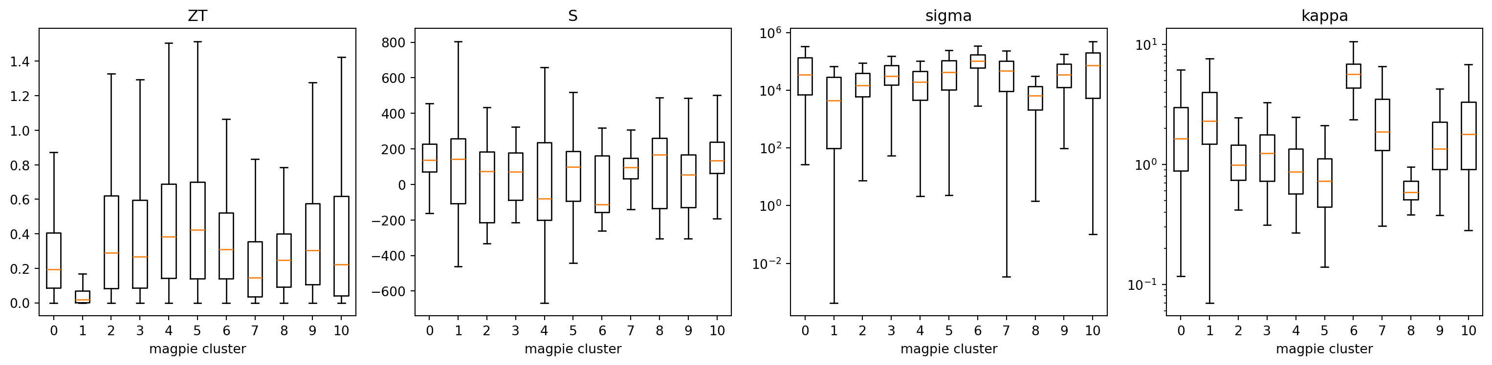
- Read per-cluster property distributions as a sanity check that clusters mean something.
- Connect this workflow to materials discovery (Na & Chang 2022 / SIMD).
Setup
import os
import warnings
from collections import Counter
from pathlib import Path

import numpy as np
import pandas as pd
import matplotlib.pyplot as plt

from sklearn.cluster import KMeans
from sklearn.decomposition import PCA
from sklearn.preprocessing import StandardScaler
from sklearn.metrics import silhouette_score

from ai4mat.datasets import ESTMDataset

np.random.seed(0)
warnings.filterwarnings("ignore", category=UserWarning, module="matminer")
Slide-figure save helper
def _resolve_slide_img_dir() -> Path:
    env = os.environ.get("ESTM_SLIDE_IMG_DIR")
    target = Path(env) if env else Path(
        "../_public_presentations/ml_for_characterization_and_processing/"
        "unit05_unsupervised_learning/images/estm"
    )
    # parents=False on purpose: do NOT silently create _public_presentations/.
    if target.parent.exists():
        target.mkdir(exist_ok=True)
        return target
    fallback = Path("figs/estm")
    fallback.mkdir(parents=True, exist_ok=True)
    warnings.warn(
        f"slide-deck images parent {target.parent.resolve()} not found; "
        f"writing slide PNGs to {fallback.resolve()} instead"
    )
    return fallback

SLIDE_IMG_DIR = _resolve_slide_img_dir()

def save_slide_fig(fig, name):
    fig.savefig(SLIDE_IMG_DIR / f"{name}.png", dpi=200, bbox_inches="tight")

print(f"Slide images → {SLIDE_IMG_DIR.resolve()}")
Slide images → /home/philipp/projects/_public_presentations/ml_for_characterization_and_processing/unit05_unsupervised_learning/images/estm1. Dataset preview
ds_frac = ESTMDataset(features="fraction", standardize=True)
ds_mag = ESTMDataset(features="magpie", standardize=True)
print(f"fraction: X={tuple(ds_frac.X.shape)}, y={tuple(ds_frac.y.shape)}")
print(f"magpie:   X={tuple(ds_mag.X.shape)}, y={tuple(ds_mag.y.shape)}")
print("temperature range:", ds_frac.T.min().item(), "-", ds_frac.T.max().item(), "K")
fraction: X=(5205, 119), y=(5205,)
magpie: X=(5205, 133), y=(5205,)
temperature range: 10.0 - 1275.0 Kdef _dominant_element(formula: str) -> str:
from pymatgen.core import Composition
comp = Composition(formula).fractional_composition.as_dict()
return max(comp, key=comp.get)
dom = [_dominant_element(f) for f in ds_frac.formulas]
top_elements = [e for e, _ in Counter(dom).most_common(15)]
T_bins = pd.cut(ds_frac.T.numpy(), bins=[0, 400, 600, 800, 1500],
labels=["≤400 K", "400-600 K", "600-800 K", ">800 K"])
preview = (
pd.DataFrame({"dom": dom, "Tbin": T_bins})
.query("dom in @top_elements")
.pipe(lambda d: pd.crosstab(d["dom"], d["Tbin"]))
.loc[top_elements]
)
preview| Tbin | ≤400 K | 400-600 K | 600-800 K | >800 K |
|---|---|---|---|---|
| dom | ||||
| Te | 257 | 417 | 277 | 77 |
| Se | 235 | 326 | 222 | 31 |
| Cu | 175 | 155 | 123 | 26 |
| Sb | 109 | 157 | 136 | 31 |
| S | 131 | 105 | 74 | 0 |
| O | 62 | 73 | 65 | 103 |
| Mg | 99 | 108 | 61 | 0 |
| Sn | 58 | 101 | 68 | 23 |
| Ge | 50 | 79 | 100 | 9 |
| Ag | 97 | 52 | 35 | 0 |
| Fe | 26 | 28 | 23 | 26 |
| Co | 28 | 23 | 23 | 23 |
| Yb | 15 | 20 | 19 | 31 |
| Ca | 10 | 27 | 20 | 11 |
| Tl | 30 | 33 | 4 | 0 |
2. Feature pipeline A — element fractions + T
X_frac = ds_frac.X.numpy()
pca_frac_10 = PCA(n_components=10, random_state=0).fit(X_frac)
pca_frac_2  = PCA(n_components=2,  random_state=0).fit(X_frac)
Z_frac10 = pca_frac_10.transform(X_frac)
Z_frac2  = pca_frac_2.transform(X_frac)

cumvar = np.cumsum(pca_frac_10.explained_variance_ratio_)
print(f"fraction PCA-10 cumulative variance: {cumvar[-1]:.2%}")
fraction PCA-10 cumulative variance: 29.54%3. Feature pipeline B — Magpie descriptors + T
X_mag = ds_mag.X.numpy()
pca_mag_10 = PCA(n_components=10, random_state=0).fit(X_mag)
pca_mag_2  = PCA(n_components=2,  random_state=0).fit(X_mag)
Z_mag10 = pca_mag_10.transform(X_mag)
Z_mag2  = pca_mag_2.transform(X_mag)

cumvar = np.cumsum(pca_mag_10.explained_variance_ratio_)
print(f"magpie PCA-10 cumulative variance: {cumvar[-1]:.2%}")

# Inspect top loadings of PC1/PC2 to see which Magpie descriptors dominate.
loadings = pd.DataFrame(
    pca_mag_2.components_.T,
    index=ds_mag.feature_names,
    columns=["PC1", "PC2"],
)
print("Top 5 by |PC1|:\n", loadings["PC1"].abs().nlargest(5))
print("Top 5 by |PC2|:\n", loadings["PC2"].abs().nlargest(5))
magpie PCA-10 cumulative variance: 77.58%
Top 5 by |PC1|:
MagpieData mean NdValence 0.159784
MagpieData mean NValence 0.157061
MagpieData minimum NValence 0.156264
MagpieData minimum Column 0.147491
MagpieData avg_dev Column 0.146422
Name: PC1, dtype: float32
Top 5 by |PC2|:
MagpieData mean CovalentRadius 0.171044
MagpieData mean Electronegativity 0.162910
MagpieData avg_dev SpaceGroupNumber 0.154333
MagpieData avg_dev NsValence 0.151971
MagpieData avg_dev NsUnfilled 0.151863
Name: PC2, dtype: float324. K-means + elbow / silhouette on both feature sets
def k_sweep(Z, k_values):
    inertias, sils = [], []
    for k in k_values:
        km = KMeans(n_clusters=k, n_init=10, random_state=0).fit(Z)
        inertias.append(km.inertia_)
        sils.append(silhouette_score(Z, km.labels_))
    return np.array(inertias), np.array(sils)

K_VALUES = np.arange(2, 13)
frac_inertia, frac_sil = k_sweep(Z_frac10, K_VALUES)
mag_inertia,  mag_sil  = k_sweep(Z_mag10,  K_VALUES)

K_star_frac = int(K_VALUES[np.argmax(frac_sil)])
K_star_mag  = int(K_VALUES[np.argmax(mag_sil)])
print(f"K* (fraction features) = {K_star_frac}")
print(f"K* (Magpie features)   = {K_star_mag}")
K* (fraction features) = 12
K* (Magpie features) = 11fig, axes = plt.subplots(1, 2, figsize=(11, 4))
for ax, inertia, sil, label, K_star in [
(axes[0], frac_inertia, frac_sil, "fraction", K_star_frac),
(axes[1], mag_inertia, mag_sil, "magpie", K_star_mag),
]:
ax.plot(K_VALUES, inertia / inertia.max(), "o-", label="inertia (norm.)")
ax.plot(K_VALUES, sil / sil.max(), "s-", label="silhouette (norm.)")
ax.axvline(K_star, color="k", linestyle=":", alpha=0.5, label=f"K* = {K_star}")
ax.set_title(f"{label} features")
ax.set_xlabel("K")
ax.set_xticks(K_VALUES)
ax.legend(loc="best", fontsize=9)
axes[0].set_ylabel("score (max-normalised)")
fig.tight_layout()
save_slide_fig(fig, "elbow_silhouette")
plt.show()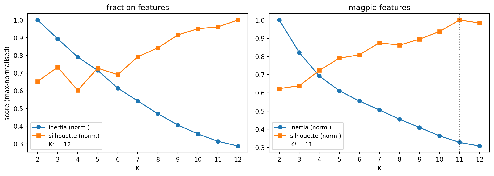
km_frac = KMeans(n_clusters=K_star_frac, n_init=10, random_state=0).fit(Z_frac10)
km_mag  = KMeans(n_clusters=K_star_mag,  n_init=10, random_state=0).fit(Z_mag10)
labels_frac = km_frac.labels_
labels_mag  = km_mag.labels_
5. Cluster visualisation in PCA space
def cluster_dominant_elements(formulas, labels) -> dict[int, str]:
    out: dict[int, str] = {}
    for c in sorted(set(labels)):
        members = [f for f, l in zip(formulas, labels) if l == c]
        elems = [_dominant_element(f) for f in members]
        out[c] = Counter(elems).most_common(1)[0][0]
    return out

dom_frac = cluster_dominant_elements(ds_frac.formulas, labels_frac)
dom_mag  = cluster_dominant_elements(ds_mag.formulas,  labels_mag)
print("fraction cluster → dominant element:", dom_frac)
print("magpie cluster   → dominant element:", dom_mag)
fraction cluster → dominant element: {0: 'Se', 1: 'Se', 2: 'Zr', 3: 'Te', 4: 'Te', 5: 'Sb', 6: 'O', 7: 'Cu', 8: 'O', 9: 'Ge', 10: 'Co', 11: 'Fe'}
magpie cluster → dominant element: {0: 'Se', 1: 'O', 2: 'Mg', 3: 'Te', 4: 'Te', 5: 'Cu', 6: 'Fe', 7: 'S', 8: 'Cu', 9: 'Sb', 10: 'Te'}def scatter_clusters(ax, Z2, labels, centroids_2d, dom_map, title):
cmap = plt.cm.tab10
for c in sorted(set(labels)):
m = labels == c
ax.scatter(Z2[m, 0], Z2[m, 1], s=6, alpha=0.5,
color=cmap(c % 10), label=f"{c}: {dom_map[c]}")
ax.scatter(centroids_2d[:, 0], centroids_2d[:, 1],
s=180, marker="*", color="black", edgecolors="white", linewidths=1.2)
for c, (cx, cy) in enumerate(centroids_2d):
ax.annotate(dom_map[c], (cx, cy), textcoords="offset points",
xytext=(6, 6), fontsize=10, weight="bold")
ax.set_xlabel("PC1")
ax.set_ylabel("PC2")
ax.set_title(title)
ax.legend(loc="best", fontsize=8, markerscale=2)
# Centroids of the 10-D clusters projected into 2-D PCA space.
cent_frac_2d = pca_frac_2.transform(
pca_frac_10.inverse_transform(km_frac.cluster_centers_)
)
cent_mag_2d = pca_mag_2.transform(
pca_mag_10.inverse_transform(km_mag.cluster_centers_)
)
fig, ax = plt.subplots(figsize=(7, 6))
scatter_clusters(ax, Z_frac2, labels_frac, cent_frac_2d, dom_frac,
"Element-fraction features — K-means clusters")
fig.tight_layout()
save_slide_fig(fig, "pca_scatter_fraction")
plt.show()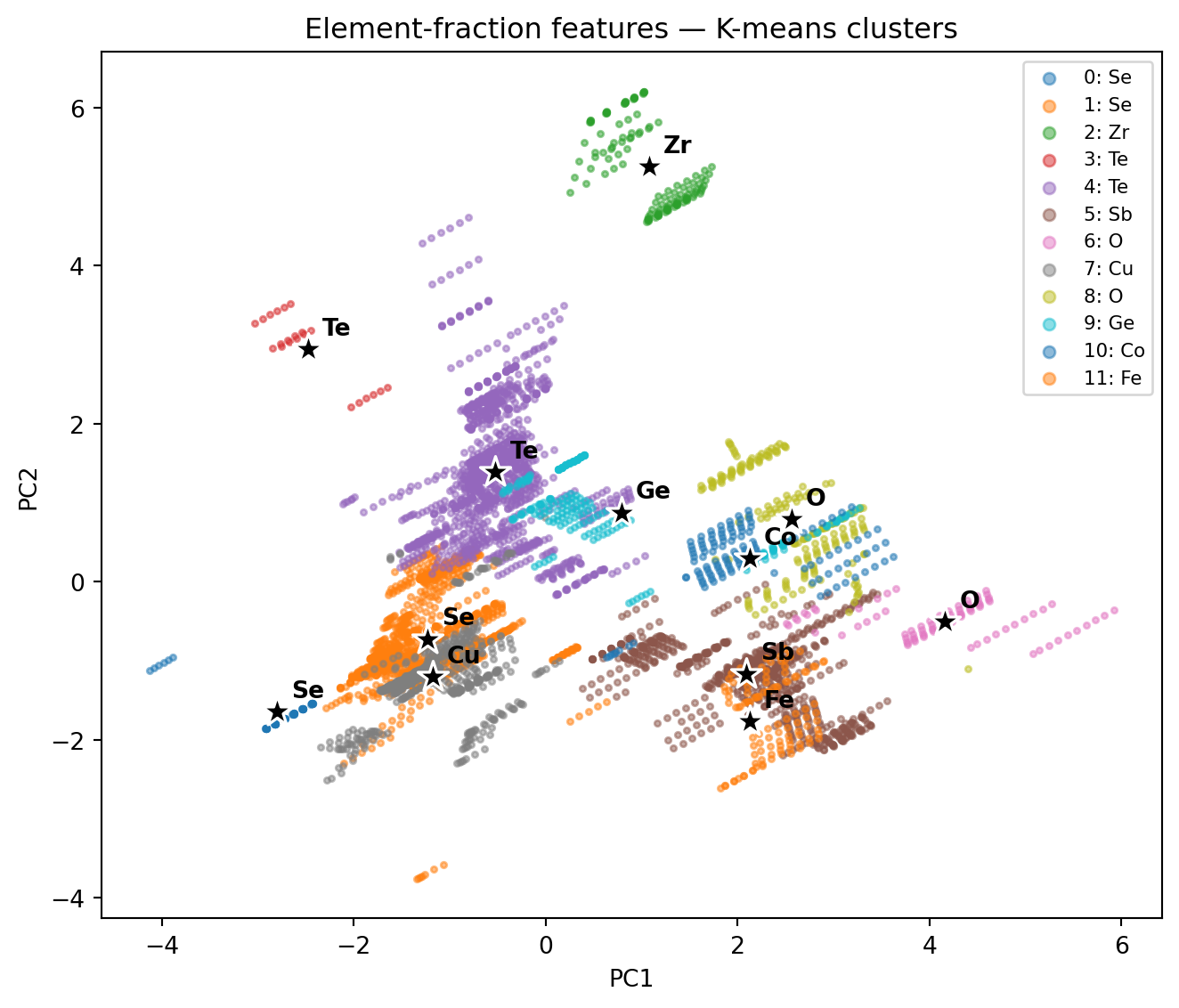
fig, ax = plt.subplots(figsize=(7, 6))
scatter_clusters(ax, Z_mag2, labels_mag, cent_mag_2d, dom_mag,
                 "Magpie features — K-means clusters")
fig.tight_layout()
save_slide_fig(fig, "pca_scatter_magpie")
plt.show()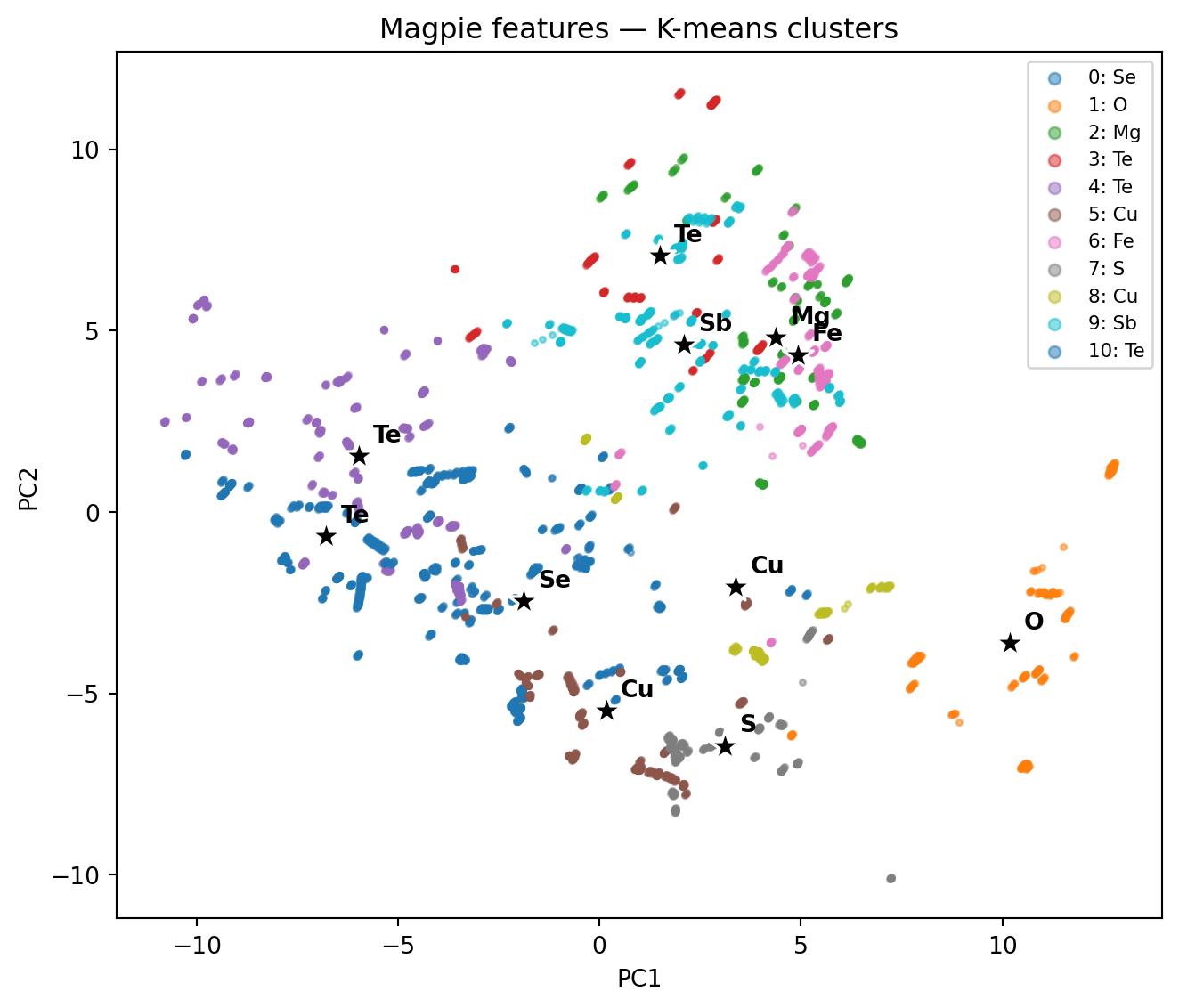
ZT_vals = ds_frac.properties["ZT"].to_numpy()
vmin, vmax = 0.0, float(np.nanquantile(ZT_vals, 0.99))
fig, axes = plt.subplots(1, 2, figsize=(12, 5))
for ax, Z2, title in [
    (axes[0], Z_frac2, "fraction features"),
    (axes[1], Z_mag2,  "magpie features"),
]:
    sc = ax.scatter(Z2[:, 0], Z2[:, 1], c=ZT_vals, s=8, alpha=0.7,
                    cmap="viridis", vmin=vmin, vmax=vmax)
    ax.set_xlabel("PC1")
    ax.set_ylabel("PC2")
    ax.set_title(title)
fig.colorbar(sc, ax=axes, label="ZT", shrink=0.85)
save_slide_fig(fig, "pca_scatter_by_zt")
plt.show()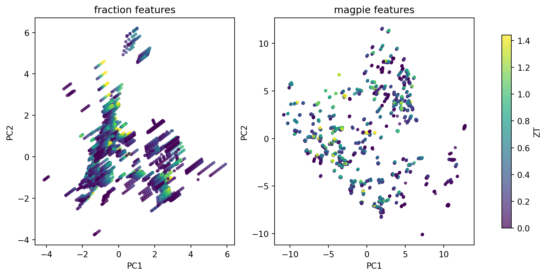
6. Per-cluster material families and property enrichment
def top_elements_per_cluster(formulas, labels, n=5):
    rows = []
    for c in sorted(set(labels)):
        members = [f for f, l in zip(formulas, labels) if l == c]
        elems = Counter(_dominant_element(f) for f in members).most_common(n)
        rows.append({"cluster": c, "n": len(members),
                     "top_elements": ", ".join(f"{e}({k})" for e, k in elems)})
    return pd.DataFrame(rows)

summary = top_elements_per_cluster(ds_mag.formulas, labels_mag, n=5).set_index("cluster")
for col in ["ZT", "S", "sigma", "kappa", "PF"]:
    summary[f"median_{col}"] = (
        pd.Series(ds_mag.properties[col].to_numpy())
          .groupby(labels_mag).median().values
    )
summary| n | top_elements | median_ZT | median_S | median_sigma | median_kappa | median_PF | |
|---|---|---|---|---|---|---|---|
| cluster | |||||||
| 0 | 933 | Se(451), Te(353), Sn(47), Ge(36), Sb(33) | 0.193800 | 137.020004 | 34000.0 | 1.64000 | 0.000583 |
| 1 | 303 | O(303) | 0.018128 | 142.000000 | 4340.0 | 2.30600 | 0.000105 |
| 2 | 389 | Mg(268), Ca(68), Yb(39), Sr(8), Si(6) | 0.291462 | 74.550003 | 14931.0 | 0.98700 | 0.000678 |
| 3 | 223 | Te(73), Yb(46), Se(36), Sb(30), Eu(22) | 0.268236 | 71.400002 | 31077.0 | 1.23700 | 0.000574 |
| 4 | 796 | Te(349), Se(258), Tl(67), In(36), Pb(36) | 0.384198 | -79.464996 | 19377.0 | 0.86950 | 0.000671 |
| 5 | 549 | Cu(365), Ag(184) | 0.422978 | 97.699997 | 41130.0 | 0.72400 | 0.000577 |
| 6 | 388 | Fe(103), Co(97), Zr(59), Nb(49), Ni(42) | 0.308769 | -112.274994 | 102373.5 | 5.62600 | 0.002496 |
| 7 | 297 | S(290), Cr(7) | 0.145585 | 95.279999 | 47000.0 | 1.86100 | 0.000636 |
| 8 | 216 | Cu(114), Se(60), Bi(42) | 0.246605 | 167.350006 | 6419.5 | 0.58485 | 0.000277 |
| 9 | 593 | Sb(352), Ge(86), Te(50), Sn(38), Zn(36) | 0.305445 | 53.869999 | 34301.0 | 1.35200 | 0.000736 |
| 10 | 518 | Te(203), Sn(165), Ge(110), In(19), As(12) | 0.222187 | 135.364990 | 72590.0 | 1.78815 | 0.001054 |
fig, axes = plt.subplots(1, 4, figsize=(16, 4))
prop_names = ["ZT", "S", "sigma", "kappa"]
log_axes = {"sigma": True, "kappa": True}
for ax, p in zip(axes, prop_names):
    data = [
        ds_mag.properties[p].to_numpy()[labels_mag == c]
        for c in sorted(set(labels_mag))
    ]
    ax.boxplot(data, labels=sorted(set(labels_mag)), showfliers=False)
    ax.set_title(p)
    ax.set_xlabel("magpie cluster")
    if log_axes.get(p):
        ax.set_yscale("log")
fig.tight_layout()
save_slide_fig(fig, "property_box_per_cluster")
plt.show()
/tmp/ipykernel_3514365/720096969.py:9: MatplotlibDeprecationWarning:
The 'labels' parameter of boxplot() has been renamed 'tick_labels' since Matplotlib 3.9; support for the old name will be dropped in 3.11.
/tmp/ipykernel_3514365/720096969.py:9: MatplotlibDeprecationWarning:
The 'labels' parameter of boxplot() has been renamed 'tick_labels' since Matplotlib 3.9; support for the old name will be dropped in 3.11.
/tmp/ipykernel_3514365/720096969.py:9: MatplotlibDeprecationWarning:
The 'labels' parameter of boxplot() has been renamed 'tick_labels' since Matplotlib 3.9; support for the old name will be dropped in 3.11.
/tmp/ipykernel_3514365/720096969.py:9: MatplotlibDeprecationWarning:
The 'labels' parameter of boxplot() has been renamed 'tick_labels' since Matplotlib 3.9; support for the old name will be dropped in 3.11.
T_vals = ds_mag.T.numpy()
T_bins = np.array([300, 400, 500, 600, 700, 800, 900, 1100])
T_centres = 0.5 * (T_bins[:-1] + T_bins[1:])

fig, ax = plt.subplots(figsize=(8, 5))
ZT = ds_mag.properties["ZT"].to_numpy()
for c in sorted(set(labels_mag)):
    m = labels_mag == c
    if m.sum() < 20:
        continue
    bin_id = np.digitize(T_vals[m], T_bins) - 1
    medians = [
        np.nanmedian(ZT[m][bin_id == b]) if (bin_id == b).any() else np.nan
        for b in range(len(T_centres))
    ]
    ax.plot(T_centres, medians, "o-", label=f"cluster {c} ({dom_mag[c]})")
ax.set_xlabel("Temperature (K)")
ax.set_ylabel("median ZT")
ax.set_title("Median ZT vs T, per Magpie cluster")
ax.legend(fontsize=9)
fig.tight_layout()
save_slide_fig(fig, "zt_by_cluster_vs_T")
plt.show()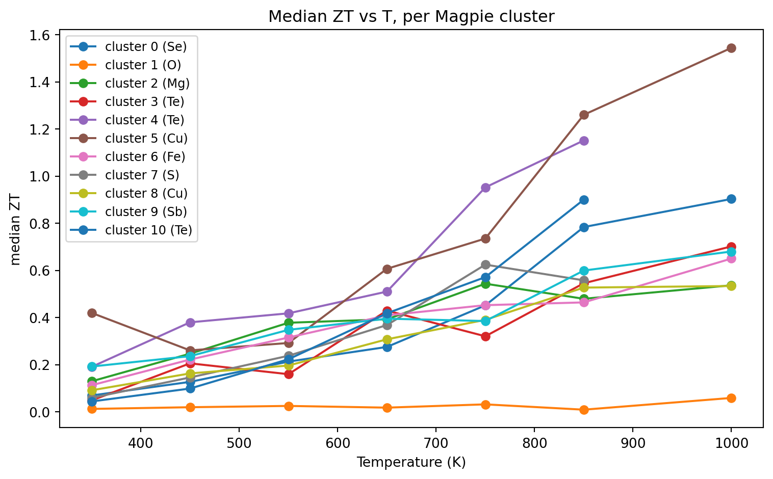
7. Wrap-up
Takeaways
- Featurization choice dominates the cluster structure. Magpie descriptors separate chalcogenides from skutterudites / half-Heuslers cleanly; raw element-fraction features mostly recover “which element is dominant” and miss subtler family structure.
- Cluster identity correlates with high ZT. A small number of Magpie clusters concentrate the top-decile ZT entries — exactly the materials- discovery signal we want from unsupervised methods.
- This is one step short of Na & Chang’s SIMD. Their representation learns a clustering-aware projection from a graph over similar materials. Magpie + K-means is the unsupervised baseline; SIMD is the natural follow-up if you want to extrapolate beyond seen families.
References
- Na, G. S. & Chang, H. npj Comput. Mater. 8, 214 (2022). DOI: 10.1038/s41524-022-00897-2
- Ward, L. et al. npj Comput. Mater. 2, 16028 (2016) — Magpie descriptors.