MLPC Week 5: Clustering steel-surface defects (NEU-DET)

K-means vs GMM on raw pixels and ResNet18 embeddings

Open In Colab

Learning Objectives

• Recognise when clustering recovers real structure vs spurious groups.
• Compare raw-pixel features to pretrained CNN embeddings on the same task.
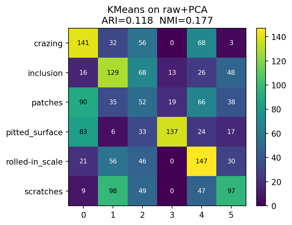
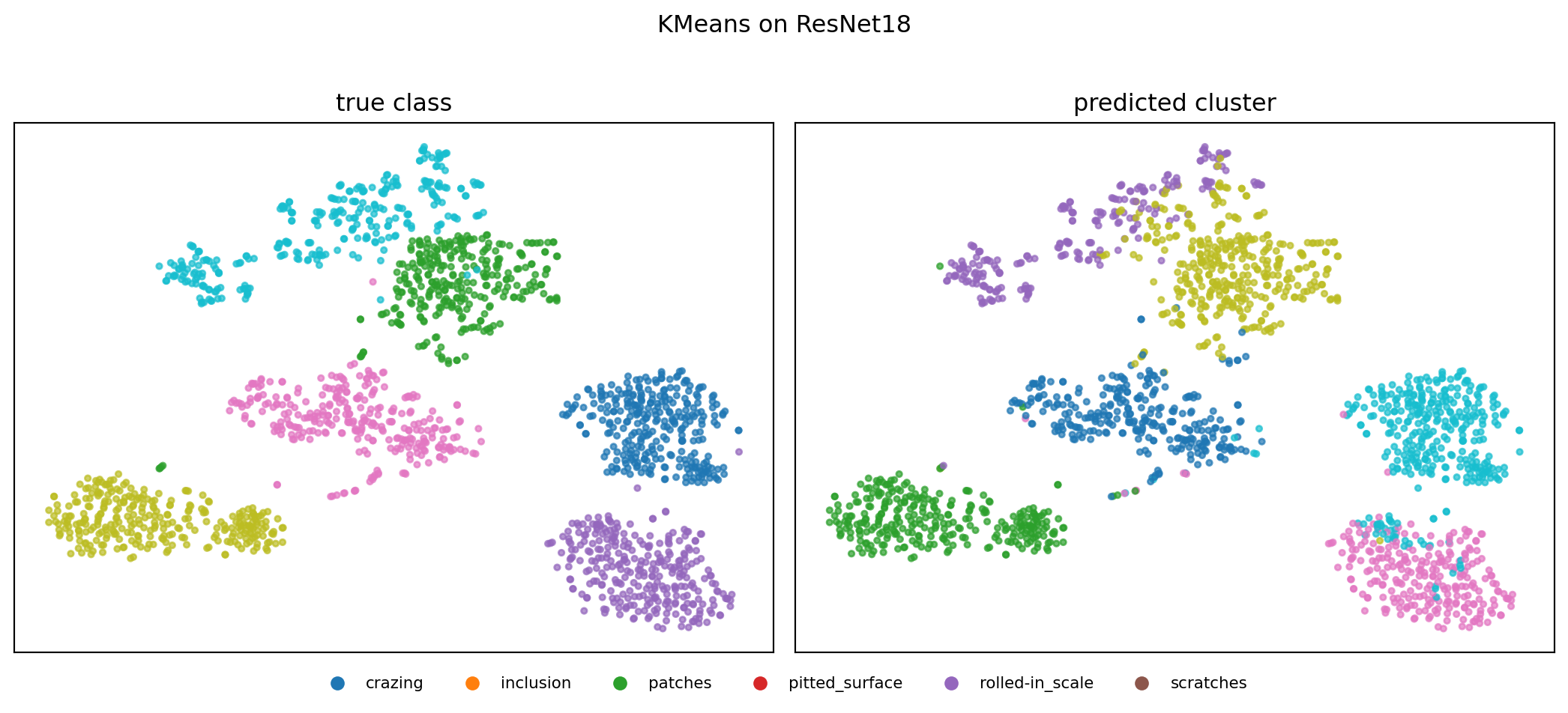
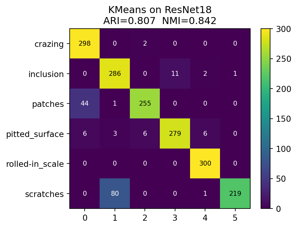
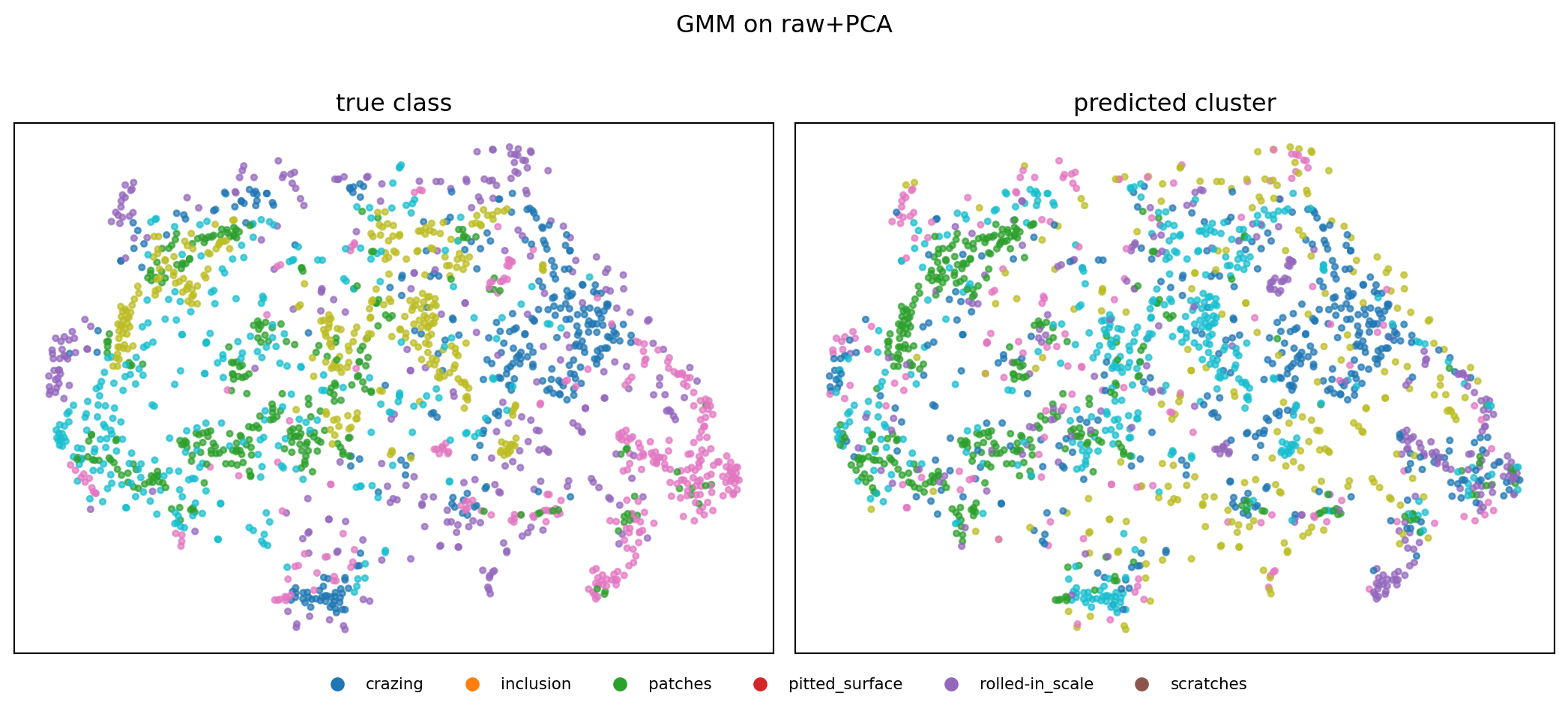
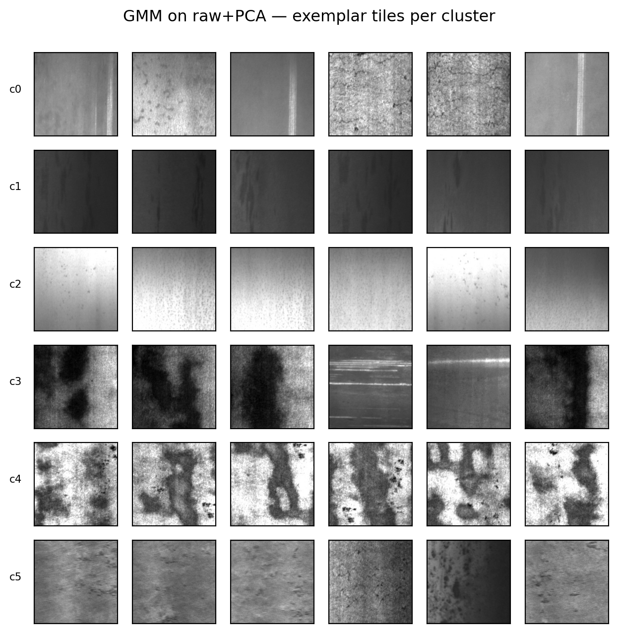
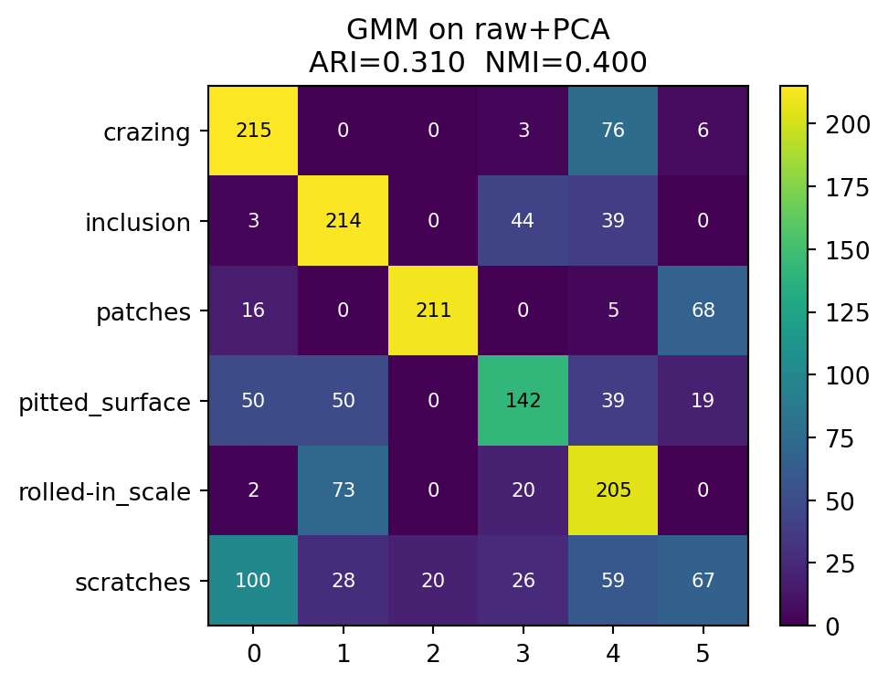
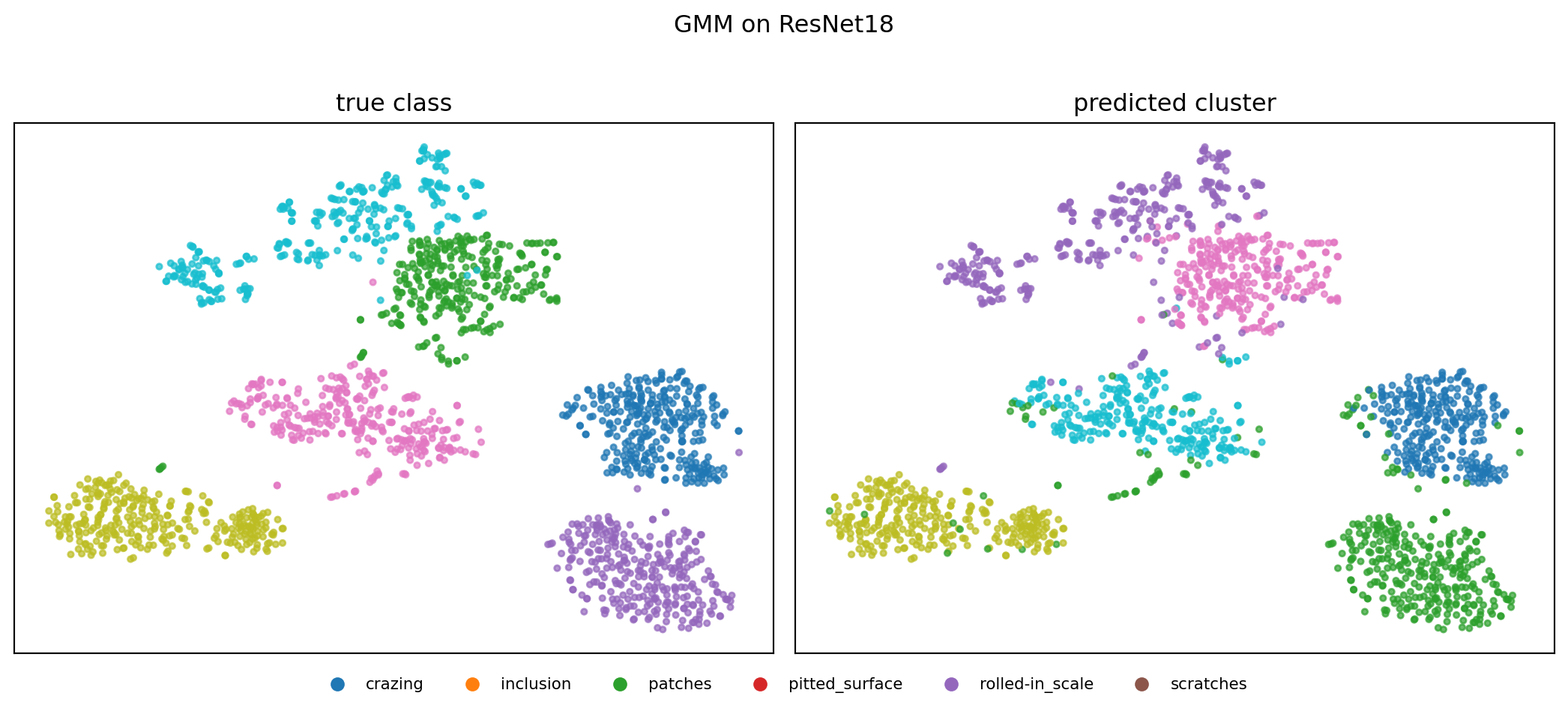
• Read t-SNE scatters, contingency matrices and ARI/NMI together.
• Connect K-means and GMM/EM (MFML Unit 5) to a real defect-classification setting.

Setup

!pip install git+https://github.com/ECLIPSE-Lab/Ai4MatLectures.git "mdsdata>=0.1.5" "torchvision>=0.16"

import os
import numpy as np
import torch
import torch.nn as nn
import torch.nn.functional as F
import matplotlib.pyplot as plt
import pandas as pd

from sklearn.cluster import KMeans
from sklearn.mixture import GaussianMixture
from sklearn.decomposition import PCA
from sklearn.manifold import TSNE
from sklearn.metrics import adjusted_rand_score, normalized_mutual_info_score, silhouette_score
from scipy.optimize import linear_sum_assignment

from ai4mat.datasets import NEUDETDataset

np.random.seed(0)
torch.manual_seed(0)
DEVICE = "cuda" if torch.cuda.is_available() else "cpu"
print(f"device: {DEVICE}")

device: cuda

1. Data preview

ds = NEUDETDataset()
print(f"N = {len(ds)}, X shape = {tuple(ds.X.shape)}, classes = {ds.class_names}")

N = 1800, X shape = (1800, 1, 200, 200), classes = ['crazing', 'inclusion', 'patches', 'pitted_surface', 'rolled-in_scale', 'scratches']

fig, axes = plt.subplots(6, 6, figsize=(10, 10))
rng = np.random.default_rng(0)
for c_idx, cls in enumerate(ds.class_names):
    idxs_in_class = np.where(ds.y.numpy() == c_idx)[0]
    picks = rng.choice(idxs_in_class, 6, replace=False)
    for j, k in enumerate(picks):
        ax = axes[c_idx, j]
        ax.imshow(ds.X[k, 0].numpy(), cmap="gray", vmin=0, vmax=1)
        ax.axis("off")
        if j == 0:
            ax.set_ylabel(cls, fontsize=9, rotation=0, labelpad=40, ha="right")
plt.suptitle("NEU-DET — 6 random examples per defect class", y=0.92)
plt.tight_layout()
plt.show()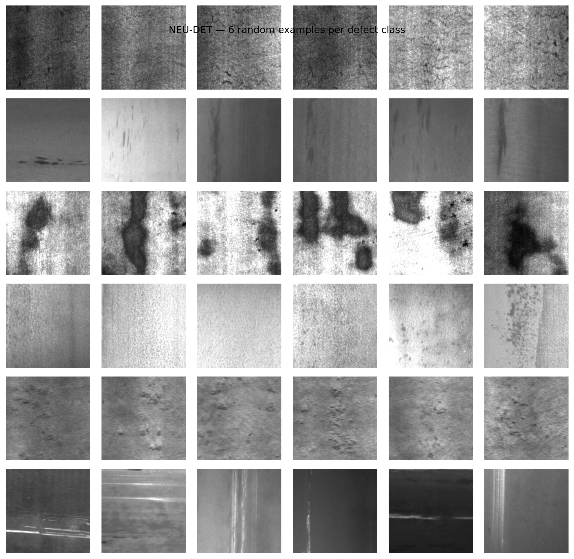

2. Feature pipeline A — raw pixels + PCA(50)

X_flat = ds.X.reshape(len(ds), -1).numpy()           # (1800, 40000)
X_flat_std = (X_flat - X_flat.mean(axis=0)) / (X_flat.std(axis=0) + 1e-8)

pca = PCA(n_components=50, random_state=0)
Z_pca = pca.fit_transform(X_flat_std)                # (1800, 50)
print(f"Z_pca shape: {Z_pca.shape}")
print(f"Cumulative explained variance @ 50 comps: {pca.explained_variance_ratio_.sum():.3f}")

Z_pca shape: (1800, 50)
Cumulative explained variance @ 50 comps: 0.926

plt.figure(figsize=(6, 3.5))
plt.plot(np.arange(1, 51), np.cumsum(pca.explained_variance_ratio_), marker="o", ms=3)
plt.xlabel("PCA component")
plt.ylabel("cumulative explained variance")
plt.title("Scree — raw pixels (40000-d) → PCA")
plt.grid(alpha=0.3)
plt.tight_layout()
plt.show()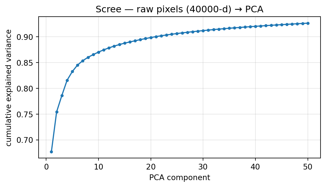

3. Feature pipeline B — pretrained ResNet18 embeddings

from torchvision import models
from torchvision.models import ResNet18_Weights

CACHE_PATH = "data/NEU-DET/embeddings_resnet18.npz"

def compute_resnet_embeddings(ds, device=DEVICE, batch_size=64):
    """Return (N, 512) float32 ResNet18 embeddings; ImageNet preprocessing."""
    backbone = models.resnet18(weights=ResNet18_Weights.IMAGENET1K_V1).to(device)
    backbone.fc = nn.Identity()
    backbone.eval()

    mean = torch.tensor([0.485, 0.456, 0.406], device=device).view(1, 3, 1, 1)
    std  = torch.tensor([0.229, 0.224, 0.225], device=device).view(1, 3, 1, 1)

    out = []
    with torch.no_grad():
        for i in range(0, len(ds), batch_size):
            x = ds.X[i : i + batch_size].to(device)        # (B, 1, 200, 200)
            x = F.interpolate(x, size=224, mode="bilinear", align_corners=False)
            x = x.expand(-1, 3, -1, -1)                    # gray -> 3 channels
            x = (x - mean) / std
            z = backbone(x)                                # (B, 512)
            out.append(z.cpu())
    return torch.cat(out).numpy()

if os.path.exists(CACHE_PATH):
    Z_resnet = np.load(CACHE_PATH)["Z"]
    print(f"Loaded cached embeddings: {Z_resnet.shape}")
else:
    Z_resnet = compute_resnet_embeddings(ds)
    np.savez(CACHE_PATH, Z=Z_resnet)
    print(f"Computed + cached embeddings: {Z_resnet.shape}")

Z_resnet_std = (Z_resnet - Z_resnet.mean(axis=0)) / (Z_resnet.std(axis=0) + 1e-8)

Loaded cached embeddings: (1800, 512)

Helpers — plot routines used across both features × both algorithms

def hungarian_remap(y_true, y_pred, K):
    """Return a permutation `perm` of cluster ids so that the diagonal of
    crosstab(y_true, perm[y_pred]) is maximal. Used for visual alignment
    only; metrics like ARI/NMI are permutation-invariant.

    Assumes the number of predicted clusters equals the number of true
    classes (the case throughout this notebook). For unequal counts you'd
    need to handle leftover rows/columns separately.
    """
    K_true = int(y_true.max()) + 1
    assert K == K_true, (
        f"hungarian_remap assumes K==K_true; got K={K}, K_true={K_true}"
    )
    C = np.zeros((K, K_true), dtype=int)
    for k in range(K):
        for c in range(K_true):
            C[k, c] = int(((y_pred == k) & (y_true == c)).sum())
    # Maximise diagonal -> minimise -C
    row_ind, col_ind = linear_sum_assignment(-C)
    perm = np.zeros(K, dtype=int)
    perm[row_ind] = col_ind
    return perm

def plot_tsne_dual(Z2, y_true, y_pred, class_names, title):
    fig, axes = plt.subplots(1, 2, figsize=(11, 4.5))
    for ax, lbl, name in zip(axes, [y_true, y_pred], ["true class", "predicted cluster"]):
        sc = ax.scatter(Z2[:, 0], Z2[:, 1], c=lbl, cmap="tab10", s=8, alpha=0.7)
        ax.set_title(f"{name}")
        ax.set_xticks([]); ax.set_yticks([])
    plt.suptitle(title, y=1.02)
    if len(class_names) <= 10:
        handles = [plt.Line2D([0], [0], marker="o", linestyle="", markersize=6,
                              color=plt.cm.tab10(i)) for i in range(len(class_names))]
        fig.legend(handles, class_names, loc="lower center", ncol=len(class_names),
                   bbox_to_anchor=(0.5, -0.05), frameon=False, fontsize=8)
    plt.tight_layout()
    plt.show()

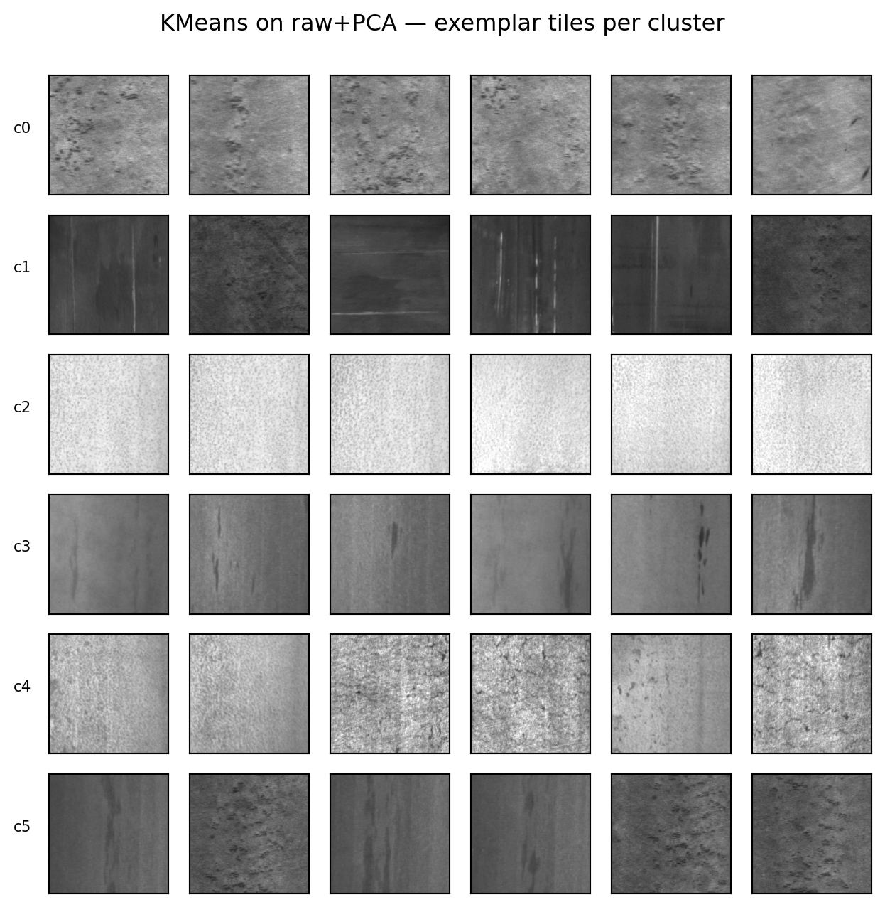
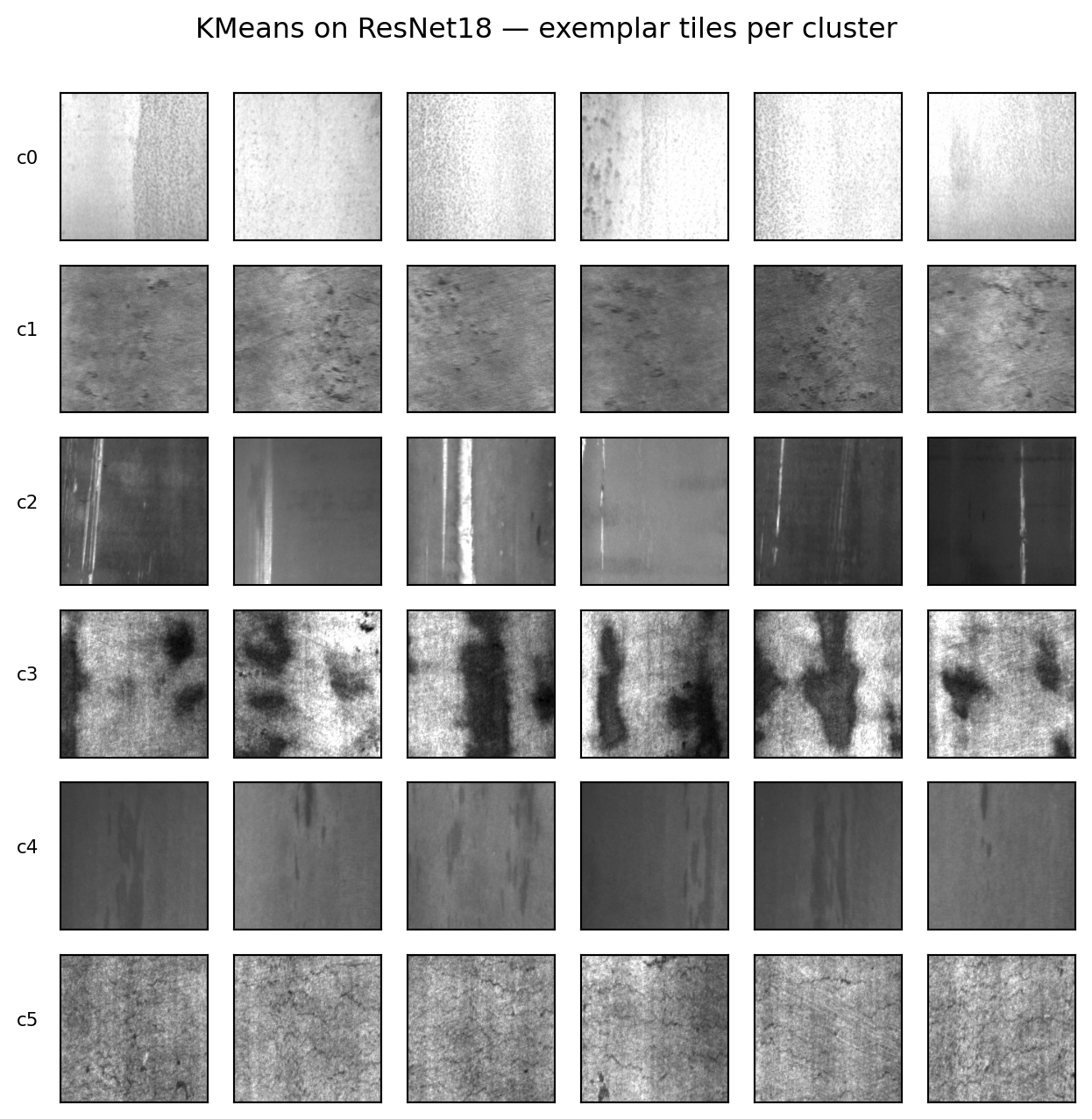
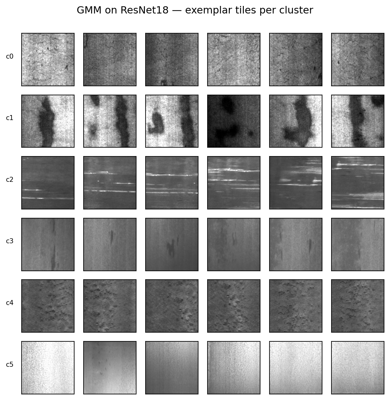
def plot_cluster_tiles(ds, y_pred, score_per_sample, n_per=6, title=""):
    """For each cluster, plot the n_per samples with the highest score
    (e.g. -dist-to-centroid for KMeans, or component responsibility for GMM)."""
    K = int(y_pred.max()) + 1
    fig, axes = plt.subplots(K, n_per, figsize=(1.1 * n_per, 1.1 * K))
    for k in range(K):
        in_cluster = np.where(y_pred == k)[0]
        order = in_cluster[np.argsort(-score_per_sample[in_cluster])]
        picks = order[:n_per]
        for j in range(n_per):
            ax = axes[k, j] if K > 1 else axes[j]
            if j < len(picks):
                ax.imshow(ds.X[picks[j], 0].numpy(), cmap="gray", vmin=0, vmax=1)
            ax.set_xticks([]); ax.set_yticks([])
            if j == 0:
                ax.set_ylabel(f"c{k}", fontsize=8, rotation=0, labelpad=14)
    plt.suptitle(title, y=1.0)
    plt.tight_layout()
    plt.show()

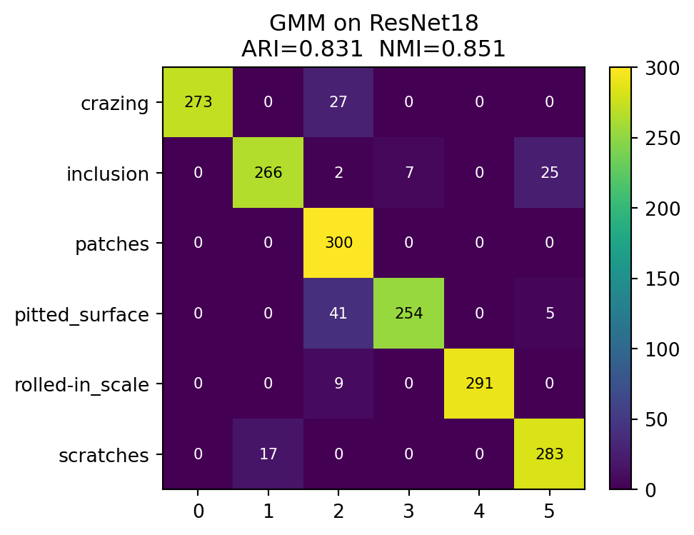
def plot_contingency(y_true, y_pred, class_names, title=""):
    K = int(y_pred.max()) + 1
    perm = hungarian_remap(y_true, y_pred, K)
    y_pred_aligned = perm[y_pred]
    df = pd.crosstab(
        pd.Series(y_true, name="true"),
        pd.Series(y_pred_aligned, name="cluster (aligned)"),
    )
    df.index = [class_names[i] for i in df.index]
    ari = adjusted_rand_score(y_true, y_pred)
    nmi = normalized_mutual_info_score(y_true, y_pred)

    fig, ax = plt.subplots(figsize=(5.5, 4))
    im = ax.imshow(df.values, cmap="viridis")
    ax.set_xticks(range(df.shape[1])); ax.set_xticklabels(df.columns)
    ax.set_yticks(range(df.shape[0])); ax.set_yticklabels(df.index)
    for i in range(df.shape[0]):
        for j in range(df.shape[1]):
            ax.text(j, i, int(df.values[i, j]), ha="center", va="center",
                    color="white" if df.values[i, j] < df.values.max() / 2 else "black",
                    fontsize=8)
    ax.set_title(f"{title}\nARI={ari:.3f}  NMI={nmi:.3f}")
    plt.colorbar(im, ax=ax, fraction=0.046, pad=0.04)
    plt.tight_layout()
    plt.show()
    return ari, nmi

4. K-means

def run_kmeans_sweep(Z, y_true, K_range=range(2, 11), seed=0):
    sil, ari = [], []
    for K in K_range:
        km = KMeans(n_clusters=K, n_init=10, random_state=seed).fit(Z)
        sil.append(silhouette_score(Z, km.labels_))
        ari.append(adjusted_rand_score(y_true, km.labels_))
    return list(K_range), sil, ari

y_true = ds.y.numpy()

for name, Z in [("raw+PCA", Z_pca), ("ResNet18", Z_resnet_std)]:
    Ks, sil, ari = run_kmeans_sweep(Z, y_true)
    fig, ax1 = plt.subplots(figsize=(6, 3.5))
    ax1.plot(Ks, sil, "o-", color="C0", label="silhouette")
    ax1.set_xlabel("K"); ax1.set_ylabel("silhouette", color="C0")
    ax2 = ax1.twinx()
    ax2.plot(Ks, ari, "s--", color="C3", label="ARI vs truth")
    ax2.set_ylabel("ARI", color="C3")
    ax1.axvline(6, color="gray", linestyle=":", alpha=0.6)
    ax1.set_title(f"K-means sweep — {name}")
    plt.tight_layout()
    plt.show()

# Fit K=6 once for each feature set and stash results.
kmeans_results = {}
for name, Z in [("raw+PCA", Z_pca), ("ResNet18", Z_resnet_std)]:
    km = KMeans(n_clusters=6, n_init=10, random_state=0).fit(Z)
    kmeans_results[name] = {
        "labels": km.labels_,
        "centroids": km.cluster_centers_,
        "Z": Z,
        # score for tile plot: higher = closer to centroid
        "score": -np.linalg.norm(Z - km.cluster_centers_[km.labels_], axis=1),
    }
    ari = adjusted_rand_score(y_true, km.labels_)
    nmi = normalized_mutual_info_score(y_true, km.labels_)
    print(f"K-means K=6 on {name:9s}: ARI={ari:.3f}  NMI={nmi:.3f}")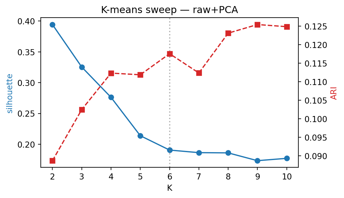

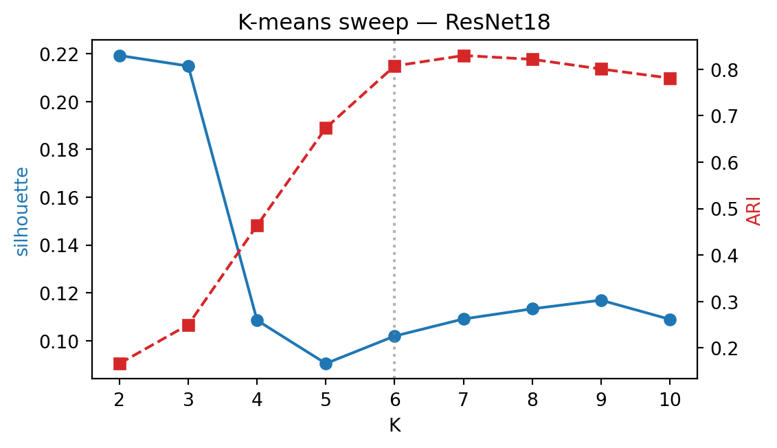
K-means K=6 on raw+PCA  : ARI=0.118  NMI=0.177
K-means K=6 on ResNet18 : ARI=0.807  NMI=0.842

5. Gaussian Mixture (EM)

def run_gmm_sweep(Z, K_range=range(2, 11), seed=0):
    bics = []
    for K in K_range:
        gm = GaussianMixture(
            n_components=K, covariance_type="diag", random_state=seed, n_init=3
        ).fit(Z)
        bics.append(gm.bic(Z))
    return list(K_range), bics

for name, Z in [("raw+PCA", Z_pca), ("ResNet18", Z_resnet_std)]:
    Ks, bics = run_gmm_sweep(Z)
    plt.figure(figsize=(6, 3.5))
    plt.plot(Ks, bics, "o-")
    plt.axvline(6, color="gray", linestyle=":", alpha=0.6)
    plt.xlabel("K"); plt.ylabel("BIC (lower = better)")
    plt.title(f"GMM BIC sweep — {name}")
    plt.tight_layout()
    plt.show()

gmm_results = {}
for name, Z in [("raw+PCA", Z_pca), ("ResNet18", Z_resnet_std)]:
    gm = GaussianMixture(
        n_components=6, covariance_type="diag", random_state=0, n_init=3
    ).fit(Z)
    labels = gm.predict(Z)
    resp = gm.predict_proba(Z)
    gmm_results[name] = {
        "labels": labels,
        "Z": Z,
        # score for tile plot: max responsibility (assignment confidence)
        "score": resp.max(axis=1),
    }
    ari = adjusted_rand_score(y_true, labels)
    nmi = normalized_mutual_info_score(y_true, labels)
    ent = -(resp * np.log(resp + 1e-12)).sum(axis=1).mean()
    print(f"GMM K=6 on {name:9s}: ARI={ari:.3f}  NMI={nmi:.3f}  mean-entropy={ent:.3f}")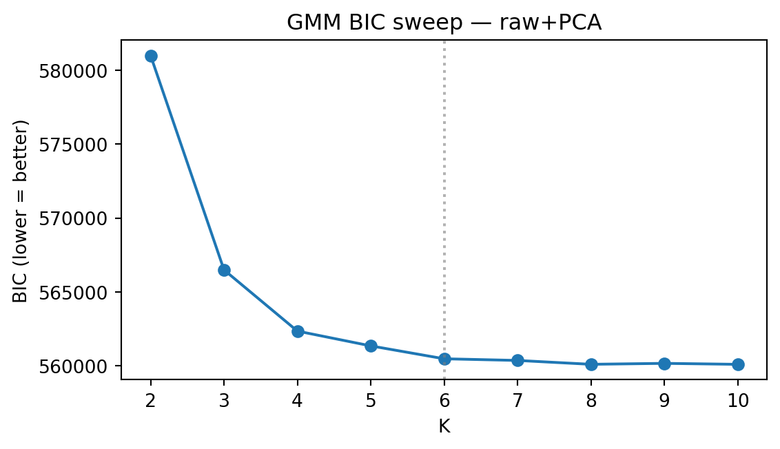

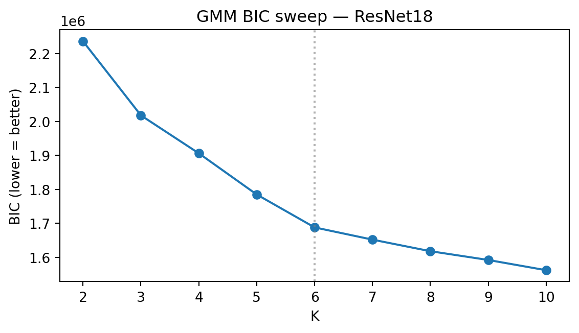
GMM K=6 on raw+PCA  : ARI=0.310  NMI=0.400  mean-entropy=0.098
GMM K=6 on ResNet18 : ARI=0.831  NMI=0.851  mean-entropy=0.000

6. Evaluation panel — t-SNE, tiles, contingency for each (features × algorithm)

# Cache t-SNE projections per feature set so we don't re-run for KMeans and GMM.
tsne_proj = {}
for name, Z in [("raw+PCA", Z_pca), ("ResNet18", Z_resnet_std)]:
    print(f"running t-SNE on {name} ...")
    tsne_proj[name] = TSNE(
        n_components=2, perplexity=30, init="pca", random_state=0
    ).fit_transform(Z)

running t-SNE on raw+PCA ...
running t-SNE on ResNet18 ...

summary_rows = []
for algo_name, results in [("KMeans", kmeans_results), ("GMM", gmm_results)]:
    for feat_name in ["raw+PCA", "ResNet18"]:
        r = results[feat_name]
        labels = r["labels"]
        Z2 = tsne_proj[feat_name]

        plot_tsne_dual(
            Z2, y_true, labels, ds.class_names,
            title=f"{algo_name} on {feat_name}",
        )
        plot_cluster_tiles(
            ds, labels, r["score"], n_per=6,
            title=f"{algo_name} on {feat_name} — exemplar tiles per cluster",
        )
        ari, nmi = plot_contingency(
            y_true, labels, ds.class_names,
            title=f"{algo_name} on {feat_name}",
        )
        summary_rows.append(
            dict(features=feat_name, algorithm=algo_name, ARI=ari, NMI=nmi)
        )

summary = pd.DataFrame(summary_rows)
summary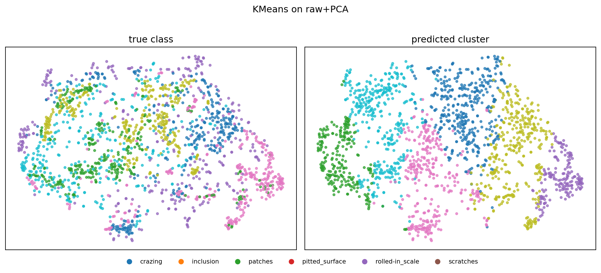

	features	algorithm	ARI	NMI
0	raw+PCA	KMeans	0.117554	0.176961
1	ResNet18	KMeans	0.807044	0.842147
2	raw+PCA	GMM	0.310175	0.399762
3	ResNet18	GMM	0.830750	0.851307

7. Wrap-up

fig, ax = plt.subplots(figsize=(7, 4))
width = 0.35
x = np.arange(len(summary))
ax.bar(x - width / 2, summary["ARI"], width, label="ARI")
ax.bar(x + width / 2, summary["NMI"], width, label="NMI")
ax.set_xticks(x)
ax.set_xticklabels([f"{r.algorithm}\n{r.features}" for r in summary.itertuples()],
                   fontsize=9)
ax.set_ylabel("score (higher = better)")
ax.set_title("Clustering quality — 4 combinations on NEU-DET")
ax.legend()
ax.grid(axis="y", alpha=0.3)
plt.tight_layout()
plt.show()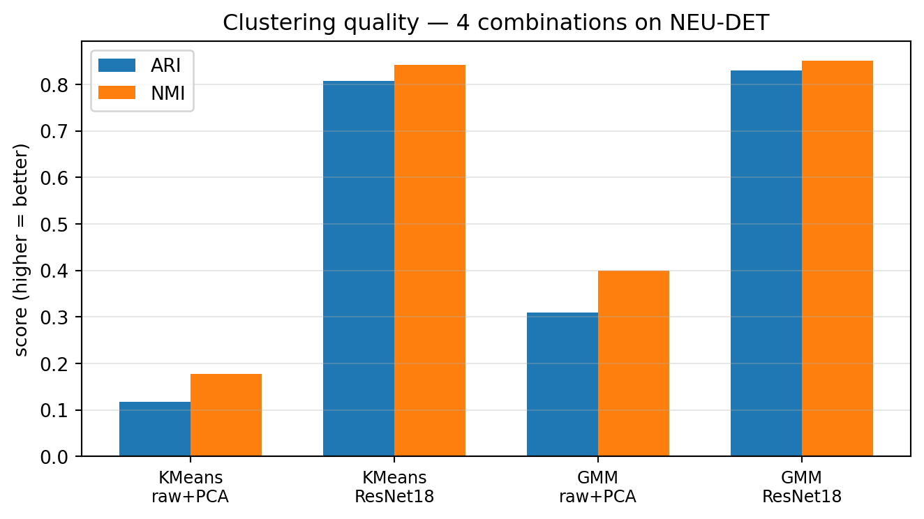

Takeaways

• Representation beats algorithm. For both KMeans and GMM, ResNet18 embeddings cluster substantially better than raw-pixel features. The features carry most of the signal; the choice between hard and soft assignment is secondary.
• Some defects are easy, others are not. Scratches and patches form visually-coherent clusters; crazing and rolled-in_scale tend to be conflated regardless of features. The contingency heatmaps make this failure mode visible at a glance.
• GMM’s soft assignments add interpretability, not accuracy here. Mean assignment entropy is informative (“which samples is the model least sure about?”) but ARI/NMI track KMeans closely.