!pip install git+https://github.com/ECLIPSE-Lab/Ai4MatLectures.git "mdsdata>=0.1.5"MLPC Week 5: CNN for 64×64 Microstructures
Scaling convolutional networks with IsingDataset (full)
![]()
Learning Objectives
- Scale a CNN architecture to larger (64×64) microstructure images
- Understand how depth and pooling affect feature map resolution
- Discuss how dataset size influences achievable accuracy
Setup
import torch
import torch.nn as nn
from torch.utils.data import DataLoader, random_split
from ai4mat.datasets import IsingDataset
import matplotlib.pyplot as plt
import numpy as np
1. Load the Data
dataset = IsingDataset(size='full')
print(f"Dataset size: {len(dataset)}")
x0, y0 = dataset[0]
print(f"Sample x shape: {x0.shape}  (C=1, H=64, W=64)")
print(f"Sample y: {y0}  (0=disordered, 1=ordered)")
Dataset size: 5000
Sample x shape: torch.Size([1, 64, 64]) (C=1, H=64, W=64)
Sample y: 0 (0=disordered, 1=ordered)fig, axes = plt.subplots(2, 5, figsize=(14, 6))
for i, ax in enumerate(axes.flat):
img = dataset[i * 500][0].squeeze().numpy()
label = dataset[i * 500][1].item()
ax.imshow(img, cmap='gray', vmin=0, vmax=1)
ax.set_title(f"{'Ordered' if label==1 else 'Disordered'}", fontsize=8)
ax.axis('off')
plt.suptitle("Ising spin configurations (64×64)")
plt.tight_layout()
plt.show()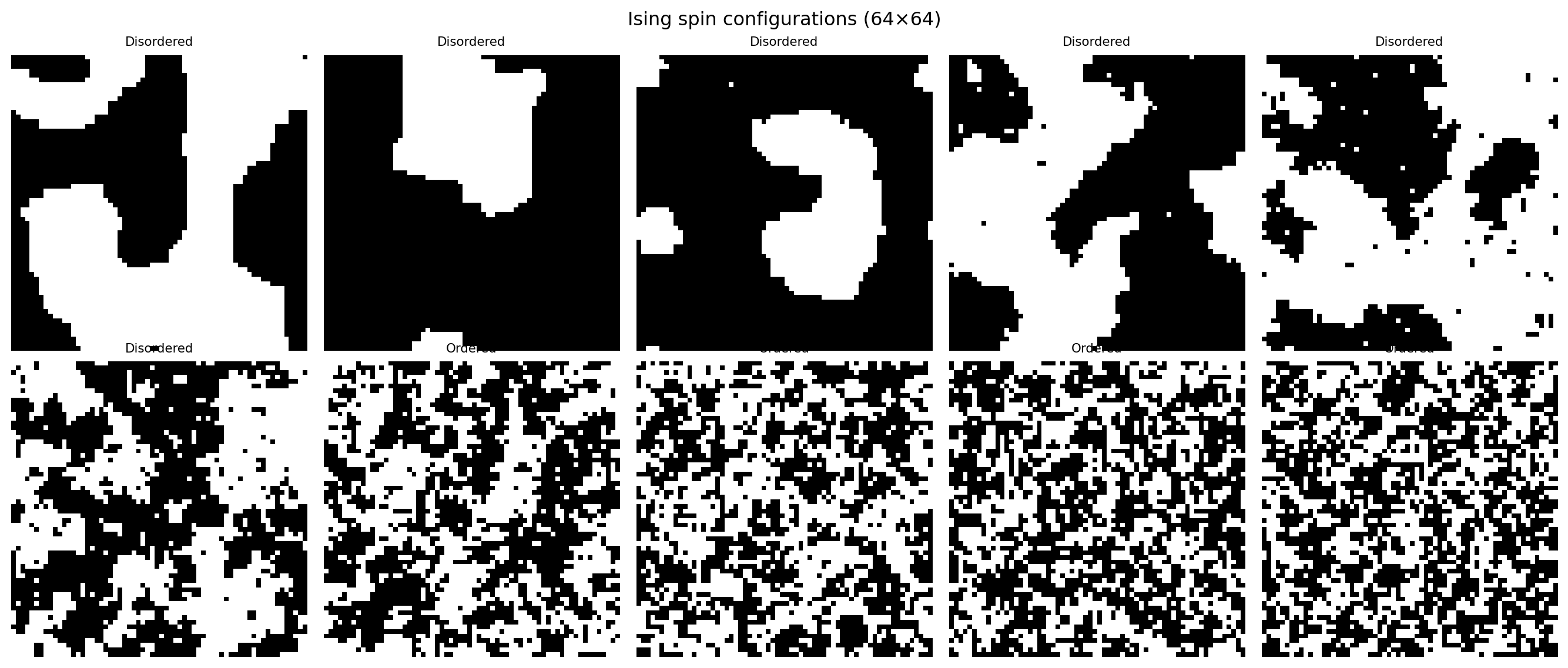
2. Train/Val Split
n_train = int(0.8 * len(dataset))
n_val = len(dataset) - n_train
train_ds, val_ds = random_split(dataset, [n_train, n_val])

train_loader = DataLoader(train_ds, batch_size=64, shuffle=True)
val_loader   = DataLoader(val_ds,   batch_size=64, shuffle=False)
print(f"Train: {n_train} | Val: {n_val}")
Train: 4000 | Val: 10003. Define the Model
class CNN(nn.Module):
    def __init__(self):
        super().__init__()
        self.features = nn.Sequential(
            nn.Conv2d(1, 16, 3, padding=1), nn.ReLU(), nn.MaxPool2d(2),   # 32x32
            nn.Conv2d(16, 32, 3, padding=1), nn.ReLU(), nn.MaxPool2d(2),  # 16x16
        )
        self.classifier = nn.Sequential(
            nn.Flatten(),
            nn.Linear(32 * 16 * 16, 64),
            nn.ReLU(),
            nn.Linear(64, 2)
        )

    def forward(self, x):
        return self.classifier(self.features(x))

model = CNN()
print(model)
print(f"\nTotal parameters: {sum(p.numel() for p in model.parameters()):,}")

# Trace feature map dimensions
x_test = torch.zeros(1, 1, 64, 64)
feat = model.features(x_test)
print(f"Feature map after 2 conv blocks: {feat.shape}  (B, C=32, H=16, W=16)")
CNN(
(features): Sequential(
(0): Conv2d(1, 16, kernel_size=(3, 3), stride=(1, 1), padding=(1, 1))
(1): ReLU()
(2): MaxPool2d(kernel_size=2, stride=2, padding=0, dilation=1, ceil_mode=False)
(3): Conv2d(16, 32, kernel_size=(3, 3), stride=(1, 1), padding=(1, 1))
(4): ReLU()
(5): MaxPool2d(kernel_size=2, stride=2, padding=0, dilation=1, ceil_mode=False)
)
(classifier): Sequential(
(0): Flatten(start_dim=1, end_dim=-1)
(1): Linear(in_features=8192, out_features=64, bias=True)
(2): ReLU()
(3): Linear(in_features=64, out_features=2, bias=True)
)
)
Total parameters: 529,282
Feature map after 2 conv blocks: torch.Size([1, 32, 16, 16]) (B, C=32, H=16, W=16)4. Training Loop
criterion = nn.CrossEntropyLoss()
optimizer = torch.optim.Adam(model.parameters(), lr=1e-3)

train_losses, val_losses = [], []
train_accs, val_accs = [], []

for epoch in range(30):
    model.train()
    ep_loss, ep_acc = 0.0, 0.0
    for x_batch, y_batch in train_loader:
        optimizer.zero_grad()
        logits = model(x_batch)
        loss = criterion(logits, y_batch)
        loss.backward()
        optimizer.step()
        ep_loss += loss.item() * len(x_batch)
        ep_acc  += (logits.argmax(1) == y_batch).float().sum().item()
    train_losses.append(ep_loss / n_train)
    train_accs.append(ep_acc / n_train)

    model.eval()
    v_loss, v_acc = 0.0, 0.0
    with torch.no_grad():
        for x_batch, y_batch in val_loader:
            logits = model(x_batch)
            v_loss += criterion(logits, y_batch).item() * len(x_batch)
            v_acc  += (logits.argmax(1) == y_batch).float().sum().item()
    val_losses.append(v_loss / n_val)
    val_accs.append(v_acc / n_val)

    if (epoch + 1) % 10 == 0:
        print(f"Epoch {epoch+1:3d} | Train acc: {train_accs[-1]:.3f} | Val acc: {val_accs[-1]:.3f}")

fig, axes = plt.subplots(1, 2, figsize=(12, 4))
axes[0].plot(train_losses, label='Train'); axes[0].plot(val_losses, label='Val')
axes[0].set_xlabel("Epoch"); axes[0].set_ylabel("Loss"); axes[0].set_title("Loss"); axes[0].legend()
axes[1].plot(train_accs, label='Train'); axes[1].plot(val_accs, label='Val')
axes[1].set_xlabel("Epoch"); axes[1].set_ylabel("Accuracy"); axes[1].set_title("Accuracy"); axes[1].legend()
plt.tight_layout(); plt.show()
print(f"\nFinal val accuracy: {val_accs[-1]:.3f}")
Epoch 10 | Train acc: 1.000 | Val acc: 0.985
Epoch 20 | Train acc: 1.000 | Val acc: 0.986
Epoch 30 | Train acc: 1.000 | Val acc: 0.985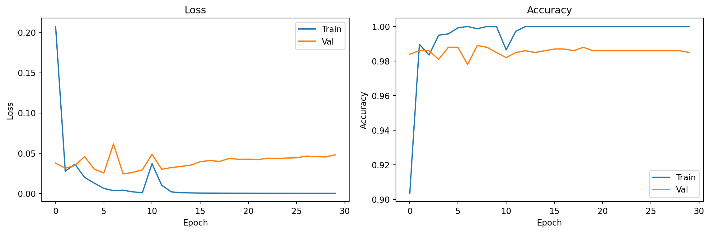
Final val accuracy: 0.9855. Evaluation
# Visualize some correct and incorrect predictions
model.eval()
x_show = torch.stack([val_ds[i][0] for i in range(20)])
y_show = torch.tensor([val_ds[i][1] for i in range(20)])
with torch.no_grad():
    preds = model(x_show).argmax(dim=1)

correct = (preds == y_show)
fig, axes = plt.subplots(2, 10, figsize=(16, 5))
for i in range(20):
    ax = axes[i // 10, i % 10]
    ax.imshow(x_show[i].squeeze().numpy(), cmap='gray', vmin=0, vmax=1)
    color = 'green' if correct[i] else 'red'
    ax.set_title(f"T:{y_show[i].item()} P:{preds[i].item()}", color=color, fontsize=7)
    ax.axis('off')
plt.suptitle("Predictions (green=correct, red=wrong)")
plt.tight_layout()
plt.show()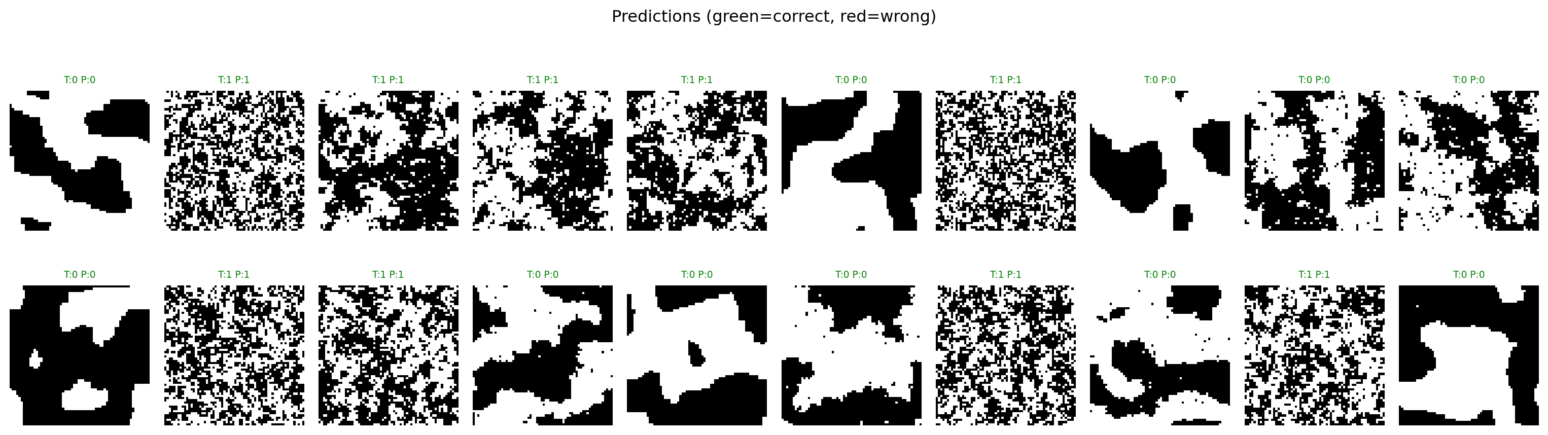
# Receptive field analysis
print("Receptive field calculation:")
print("  After Conv1 (3x3, stride 1): RF = 3")
print("  After MaxPool1 (2x2):         RF = 6")
print("  After Conv2 (3x3, stride 1): RF = 10")
print("  After MaxPool2 (2x2):         RF = 20")
print()
print("Each neuron in the final feature map 'sees' a 20×20 region of the input.")
print("For 64×64 Ising configs, this is ~10% of the total area — enough to")
print("capture local spin order patterns without seeing the whole image.")
Receptive field calculation:
After Conv1 (3x3, stride 1): RF = 3
After MaxPool1 (2x2): RF = 6
After Conv2 (3x3, stride 1): RF = 10
After MaxPool2 (2x2): RF = 20
Each neuron in the final feature map 'sees' a 20×20 region of the input.
For 64×64 Ising configs, this is ~10% of the total area — enough to
capture local spin order patterns without seeing the whole image.Exercises
- Add a third conv block:
nn.Conv2d(32, 64, 3, padding=1), nn.ReLU(), nn.MaxPool2d(2)(output: 8×8). Does accuracy improve or is it overkill for this binary task? - What is the receptive field after 2 MaxPool layers (calculation shown above)? How does this compare to the correlation length in the Ising model near Tc?
- Reduce the training data to 500 samples:
train_ds_small, _ = random_split(dataset, [500, len(dataset)-500]). How fast does accuracy drop compared to using all 4000 training samples?