!pip install git+https://github.com/ECLIPSE-Lab/Ai4MatLectures.gitMLPC Week 13: MC-Dropout uncertainty for SEM defect segmentation (MetalDAM)
Per-pixel uncertainty maps, reject-for-review curves, and tool-shift calibration

Companion to the Week-13 self-study deck (unit 12, §D). Same dataset, same method, smaller model and fewer epochs so it runs in minutes — expect the same qualitative behaviour as the lecture figures, not identical numbers.
Learning Objectives
- Turn a deterministic U-Net into an MC-Dropout model and keep dropout on at inference (the
model.eval()trap). - Read a per-pixel predictive-entropy map: where the model hesitates and why.
- Build a reject-for-human-review operating curve and understand why its ceiling is set by confidently wrong pixels.
- Audit calibration with reliability diagrams under a (simulated) SEM tool shift, and fix the confidences — not the model — with temperature scaling.
Setup
import numpy as np
import torch
import torch.nn as nn
import torch.nn.functional as F
import matplotlib.pyplot as plt
from matplotlib.colors import ListedColormap

from ai4mat.datasets import MetalDAMDataset

rng = np.random.default_rng(0)
torch.manual_seed(0)
DEVICE = "cuda" if torch.cuda.is_available() else "cpu"
print(f"device: {DEVICE}")
device: cuda1. MetalDAM: 42 SEM micrographs, 5 classes, brutal imbalance
MetalDAM (ArcelorMittal / DaSCI) is a per-pixel segmentation set of additively manufactured steel. tile_size=256 cuts the micrographs into uniform tiles for batching; tile_image_index remembers which micrograph each tile came from — split by micrograph, never by tile, or overlapping texture leaks between train and test.
ds = MetalDAMDataset(tile_size=256)
print(f"{len(ds.images)} micrographs -> {len(ds)} tiles of 256x256")

freq = np.bincount(ds.y.numpy().ravel(), minlength=5) / ds.y.numel()
for name, f in zip(ds.class_names, freq):
    print(f"  {name:22s} {100*f:6.2f}%")
42 micrographs -> 552 tiles of 256x256
matrix 34.68%
austenite 55.48%
martensite_austenite 8.92%
precipitate 0.23%
defect 0.69%order = rng.permutation(len(ds.images))
train_imgs, cal_imgs, test_imgs = order[:30], order[30:34], order[34:]
owner = ds.tile_image_index.numpy()
train_tiles = np.isin(owner, train_imgs)
Xtr, ytr = ds.X[train_tiles], ds.y[train_tiles]
print(f"train {len(train_imgs)} / calibration {len(cal_imgs)} / test {len(test_imgs)} micrographs")
print(f"train tiles: {len(Xtr)}")train 30 / calibration 4 / test 8 micrographs
train tiles: 3922. A small U-Net with dropout where it matters
Dropout (\(p=0.2\)) goes in the bottleneck and decoder blocks — early encoder dropout destroys low-level features, output-layer dropout gives near-zero variance because the class decision is already made.
class Block(nn.Module):
    def __init__(self, cin, cout, p_drop=0.0):
        super().__init__()
        layers = [
            nn.Conv2d(cin, cout, 3, padding=1), nn.BatchNorm2d(cout), nn.ReLU(inplace=True),
            nn.Conv2d(cout, cout, 3, padding=1), nn.BatchNorm2d(cout), nn.ReLU(inplace=True),
        ]
        if p_drop > 0:
            layers.append(nn.Dropout2d(p_drop))
        self.net = nn.Sequential(*layers)

    def forward(self, x):
        return self.net(x)


class UNet(nn.Module):
    def __init__(self, n_cls=5, base=16, p_drop=0.2):
        super().__init__()
        b = base
        self.e1, self.e2, self.e3 = Block(1, b), Block(b, 2 * b), Block(2 * b, 4 * b)
        self.bott = Block(4 * b, 8 * b, p_drop)
        self.up3, self.d3 = nn.ConvTranspose2d(8 * b, 4 * b, 2, 2), Block(8 * b, 4 * b, p_drop)
        self.up2, self.d2 = nn.ConvTranspose2d(4 * b, 2 * b, 2, 2), Block(4 * b, 2 * b, p_drop)
        self.up1, self.d1 = nn.ConvTranspose2d(2 * b, b, 2, 2), Block(2 * b, b, p_drop)
        self.head = nn.Conv2d(b, n_cls, 1)
        self.pool = nn.MaxPool2d(2)

    def forward(self, x):
        e1 = self.e1(x)
        e2 = self.e2(self.pool(e1))
        e3 = self.e3(self.pool(e2))
        bt = self.bott(self.pool(e3))
        d3 = self.d3(torch.cat([self.up3(bt), e3], 1))
        d2 = self.d2(torch.cat([self.up2(d3), e2], 1))
        d1 = self.d1(torch.cat([self.up1(d2), e1], 1))
        return self.head(d1)


model = UNet().to(DEVICE)
print(sum(p.numel() for p in model.parameters()) / 1e6, "M parameters")
0.483221 M parameters3. Train with a class-weighted loss
Defect pixels are 0.7% of the data — unweighted cross-entropy would learn to ignore them.
w = 1.0 / np.sqrt(freq + 1e-6)
w = w / w.sum() * 5
crit = nn.CrossEntropyLoss(weight=torch.tensor(w, dtype=torch.float32, device=DEVICE))
opt = torch.optim.Adam(model.parameters(), lr=1e-3)

EPOCHS, BS = 12, 16
n = len(Xtr)
for ep in range(EPOCHS):
    model.train()
    perm = rng.permutation(n)
    tot = 0.0
    for i in range(0, n, BS):
        idx = perm[i : i + BS]
        xb, yb = Xtr[idx].to(DEVICE), ytr[idx].to(DEVICE)
        if rng.random() < 0.5:                      # cheap augmentation
            xb, yb = torch.flip(xb, (3,)), torch.flip(yb, (2,))
        opt.zero_grad()
        loss = crit(model(xb), yb)
        loss.backward()
        opt.step()
        tot += loss.item() * len(idx)
    if (ep + 1) % 3 == 0:
        print(f"epoch {ep+1:2d}  loss {tot/n:.4f}")
epoch 3 loss 1.0384
epoch 6 loss 0.8049
epoch 9 loss 0.7136
epoch 12 loss 0.65194. MC Dropout: the two lines everyone gets wrong
model.eval() freezes BatchNorm (good) and silently switches dropout off (fatal for MC Dropout). Re-enable only the dropout layers:
def enable_dropout(model):
    for m in model.modules():
        if isinstance(m, (nn.Dropout, nn.Dropout2d)):
            m.train()


@torch.no_grad()
def mc_predict(model, img, T=20, temp=1.0):
    """T stochastic passes on one full micrograph -> mean probs, mean logits."""
    H, W = img.shape
    ph, pw = (8 - H % 8) % 8, (8 - W % 8) % 8
    x = torch.from_numpy(img).float()[None, None].to(DEVICE)
    x = F.pad(x, (0, pw, 0, ph), mode="reflect")
    model.eval()
    enable_dropout(model)          # <-- the critical line
    probs = torch.zeros(5, x.shape[2], x.shape[3], device=DEVICE)
    logits = torch.zeros_like(probs)
    for _ in range(T):
        lg = model(x)[0]
        probs += F.softmax(lg / temp, dim=0)
        logits += lg
    return (probs / T)[:, :H, :W].cpu().numpy(), (logits / T)[:, :H, :W].cpu().numpy()


def entropy(p):
    return -(p * np.log(p + 1e-12)).sum(0)
5. Per-pixel uncertainty maps
CLASS_COLORS = ["#9e9e9e", "#4878a8", "#ff9d3c", "#4daf4a", "#d62728"]
CMAP = ListedColormap(CLASS_COLORS)

imgs = [im[0].numpy() for im in ds.images]
masks = [m.numpy() for m in ds.masks]

# show the test micrograph with the most defect pixels
show = max(test_imgs, key=lambda i: (masks[i] == 4).sum())
p, _ = mc_predict(model, imgs[show])
H = entropy(p) / np.log(5)

fig, axes = plt.subplots(1, 3, figsize=(15, 4))
axes[0].imshow(imgs[show], cmap="gray"); axes[0].set_title("SEM input")
axes[1].imshow(p.argmax(0), cmap=CMAP, vmin=-0.5, vmax=4.5, interpolation="nearest")
axes[1].set_title("MC-mean prediction")
im2 = axes[2].imshow(H, cmap="inferno"); axes[2].set_title("predictive entropy")
fig.colorbar(im2, ax=axes[2], fraction=0.037)
for ax in axes:
    ax.set_xticks([]); ax.set_yticks([])
handles = [plt.Rectangle((0, 0), 1, 1, fc=c) for c in CLASS_COLORS]
axes[1].legend(handles, ds.class_names, loc="upper center",
               bbox_to_anchor=(0.5, -0.05), ncol=3, fontsize=8, frameon=False)
plt.tight_layout(); plt.show()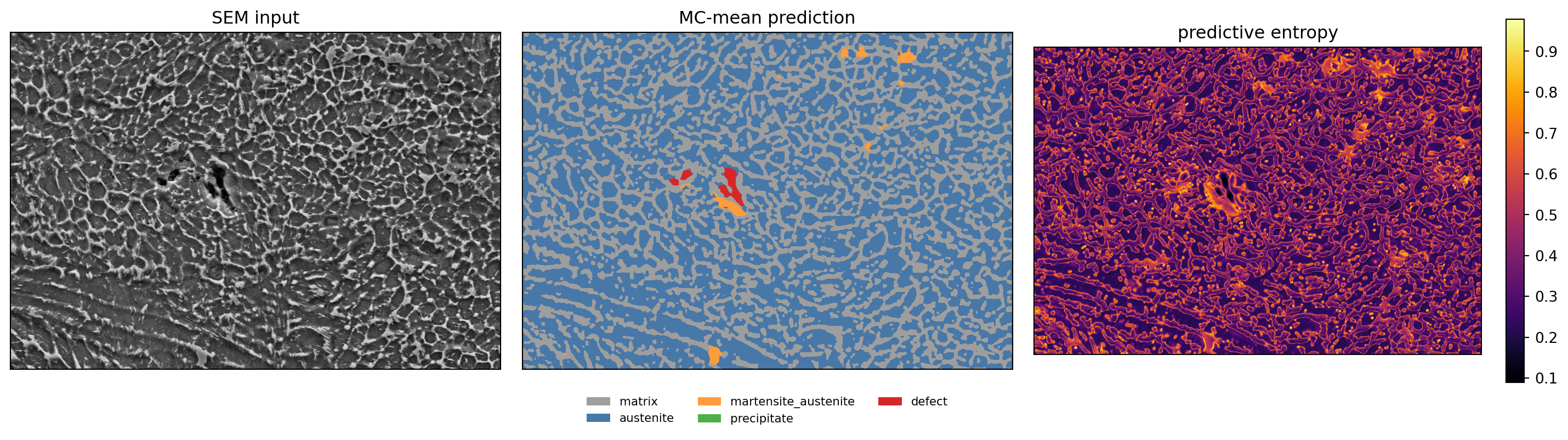
High entropy should sit on phase boundaries, inside ambiguous martensite/austenite regions, and at defect rims — the places a human expert would also zoom into.
6. Reject-for-human-review operating curve
Flag the highest-entropy pixels for an operator; auto-classify the rest. The curve is the deliverable — the operating point is a business decision (cost of a missed defect vs cost of analyst time).
probs_l, ys = [], []
for i in test_imgs:
    p, _ = mc_predict(model, imgs[i])
    probs_l.append(p); ys.append(masks[i])

Hs = np.concatenate([entropy(p).ravel() for p in probs_l])
yy = np.concatenate([y.ravel() for y in ys])
pp = np.concatenate([p.argmax(0).ravel() for p in probs_l])
is_def = yy == 4
auto_ok = (pp == 4) & is_def
auto_recall = auto_ok[is_def].mean()

order_H = np.argsort(-Hs)
qs = np.array([0.001, 0.002, 0.005, 0.01, 0.02, 0.05, 0.1, 0.2])
rec = []
flagged = np.zeros(len(Hs), bool)
for q in qs:
    flagged[:] = False
    flagged[order_H[: int(q * len(Hs))]] = True
    rec.append((auto_ok | flagged)[is_def].mean())

fig, ax = plt.subplots(figsize=(7, 4.2))
ax.axhline(auto_recall * 100, color="gray", ls="--", lw=1)
ax.plot(qs * 100, np.array(rec) * 100, "o-")
ax.set_xscale("log")
ax.set_xlabel("human-review rate (% of pixels flagged)")
ax.set_ylabel("defect-pixel recall (%)")
ax.set_title(f"fully automatic: {auto_recall*100:.1f}% — review adds the rest")
ax.grid(alpha=0.3)
plt.tight_layout(); plt.show()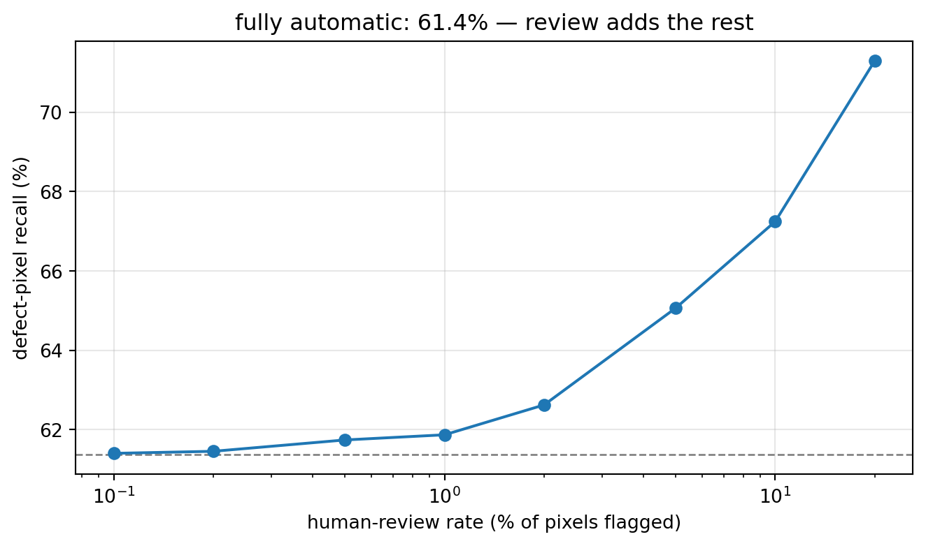
Note the gap to 100% that review cannot close: those defect pixels are confidently wrong (low entropy). No entropy threshold finds them — that is a calibration problem, which brings us to the last section.
7. Tool shift: overconfidence, and the one-scalar fix
MetalDAM comes from a single instrument, so we simulate a second SEM: different detector gamma, contrast, brightness, slight defocus, more noise. Then we audit calibration with reliability diagrams.
def simulate_tool_shift(img):
    out = np.clip(img, 0, 1) ** 0.70
    out = (out - 0.5) * 1.35 + 0.5 + 0.05
    k = np.array([0.25, 0.5, 0.25])
    out = np.apply_along_axis(lambda r: np.convolve(r, k, "same"), 1, out)
    out = np.apply_along_axis(lambda c: np.convolve(c, k, "same"), 0, out)
    return np.clip(out + rng.normal(0, 0.035, out.shape), 0, 1).astype(np.float32)


def reliability(conf, correct, n_bins=15):
    bins = np.linspace(0, 1, n_bins + 1)
    mids, accs, ece = [], [], 0.0
    for lo, hi in zip(bins[:-1], bins[1:]):
        m = (conf > lo) & (conf <= hi)
        if m.sum() == 0:
            continue
        mids.append(conf[m].mean()); accs.append(correct[m].mean())
        ece += m.mean() * abs(accs[-1] - mids[-1])
    return np.array(mids), np.array(accs), ece
Fit one temperature on a small calibration set from the new tool (here: the 4 held-out calibration micrographs), then re-run inference with scaled logits:
cal_lg, cal_y = [], []
for i in cal_imgs:
    _, lg = mc_predict(model, simulate_tool_shift(imgs[i]))
    cal_lg.append(lg.reshape(5, -1).T); cal_y.append(masks[i].ravel())
lg = torch.from_numpy(np.concatenate(cal_lg)).float().to(DEVICE)
yy_cal = torch.from_numpy(np.concatenate(cal_y)).to(DEVICE)
sub = torch.randperm(len(yy_cal))[:200_000]
lg, yy_cal = lg[sub], yy_cal[sub]

logT = torch.zeros(1, device=DEVICE, requires_grad=True)
optT = torch.optim.LBFGS([logT], lr=0.1, max_iter=50)

def closure():
    optT.zero_grad()
    loss = F.cross_entropy(lg / torch.exp(logT), yy_cal)
    loss.backward()
    return loss

optT.step(closure)
T_scal = float(torch.exp(logT))
print(f"fitted temperature: T = {T_scal:.2f}")
fitted temperature: T = 1.78panels = []
panels.append(("SEM #1 (training tool)", probs_l, ys))
shifted = [simulate_tool_shift(imgs[i]) for i in test_imgs]
p2 = [mc_predict(model, s)[0] for s in shifted]
panels.append(("SEM #2 (simulated shift)", p2, ys))
p2c = [mc_predict(model, s, temp=T_scal)[0] for s in shifted]
panels.append((f"SEM #2, temp-scaled (T={T_scal:.2f})", p2c, ys))
fig, axes = plt.subplots(1, 3, figsize=(14, 4), sharey=True)
for ax, (title, pl, yl) in zip(axes, panels):
conf = np.concatenate([p.max(0).ravel() for p in pl])
corr = np.concatenate([(p.argmax(0) == y).ravel() for p, y in zip(pl, yl)]).astype(float)
mids, accs, ece = reliability(conf, corr)
ax.bar(mids, accs, width=0.055, color="#4878a8", edgecolor="k", lw=0.4)
ax.plot([0, 1], [0, 1], "k--", lw=1)
ax.set_title(title, fontsize=11)
ax.text(0.05, 0.92, f"ECE = {ece*100:.1f}%", transform=ax.transAxes,
bbox=dict(fc="white", ec="gray", alpha=0.8))
ax.set_xlabel("confidence")
axes[0].set_ylabel("accuracy")
plt.tight_layout(); plt.show()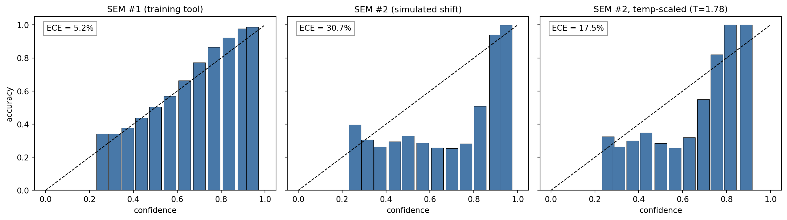
Takeaways
- The predictive mean is the prediction, the entropy is the honesty. Both come from the same \(T\) stochastic passes; forgetting
enable_dropout()silently degrades this to a deterministic model. - Review curves have a ceiling. Entropy-ranked review recovers the hesitantly wrong pixels; the confidently wrong ones are invisible to it. Report the curve, let the deployment pick the point.
- Tool shift breaks confidence before it breaks anything else. The shifted reliability diagram sags below the diagonal (overconfidence); one temperature fitted on a handful of new-tool micrographs removes a large part of that overconfidence without changing a single prediction — and without recovering the lost accuracy. (This small model keeps a residual ECE after scaling; the larger lecture model returns to training-tool level. If scaling is not enough, that is your signal the shift moved more than the confidences.) Calibration and accuracy are different failure modes; diagnose before you retrain.
Exercises
- Sweep the number of MC passes \(T \in \{2, 5, 10, 20, 40\}\) and plot ECE on the test micrographs vs \(T\). Where does it stop improving?
- Move the dropout: encoder-only vs bottleneck+decoder (as here) vs a single layer before the head. Compare the entropy maps — which placement produces uncertainty that still localises?
- The precipitate class has near-zero IoU because most precipitates were never annotated (dataset README). What does that do to its entropy? Is high entropy on precipitates a model failure or a label failure?