Week 10 — Attention, ViT, and cross-system transfer

This week braids three lectures:

MFML Unit 10 — Attention & Transformers. We turn the from-scratch multi-head attention from the homework into a tiny ViT (positional encoding + transformer blocks + classification head) and compare it against a CNN baseline of the same parameter budget.
MG Unit 9 — Neural Networks for Materials Properties. We build a graph neural network on atomic systems: a SchNet-style continuous-filter convolution and a CGCNN-style gated message-passing layer on crystal graphs, predicting formation energy. We make the four symmetries (translation, rotation, permutation, periodicity) concrete, contrast extensive (sum) vs intensive (mean) pooling, beat a composition-only Magpie+MLP baseline, and finish with the §43 pretrain → freeze → fine-tune foundation-model recipe.
ML-PC parallel-track this week. Unit 9b (Transformers for Materials) is a companion deck within W9 and pairs naturally with this notebook. ML-PC Unit 10 (Automation in microscopy) is the calendar-W10 lecture but uses different material; this notebook stays on attention/ViT and ends by running the same multi-head attention on tensile curves treated as 1D sequences — the spectral-compression analogue.

Red thread. A neural network’s job is to respect the structure of its input. For an image, attention must be told position matters (a bug fixed by positional encoding). For an unordered set of atoms in a crystal, permutation-invariant aggregation is exactly the correct symmetry — which is why GNN message passing sums/means over neighbours. Today we build a tiny ViT, watch its attention beat or tie a parameter-matched CNN, then build a real crystal-graph GNN whose continuous-filter / gated message passing predicts formation energy, and finish by running the same attention machinery on 1D tensile-curve sequences.

Pre-flight check. This notebook assumes you have run notebooks/week10_homework.py. Block 1 picks up directly from your scaled-dot-product attention function and your MultiHeadSelfAttention module; we will not re-derive them.

Agenda (90 min)

Block	Min	Topic
1	6	Recap from homework — patch attention on Ising
2	12	Positional encoding: why permutation-equivariance is a bug, not a feature
3	14	Tiny ViT: stack two transformer blocks, classify Ising; compare to a CNN
4	12	Attention maps as interpretability vs CNN input-gradient saliency
5	16	MG-U9: a crystal-graph GNN — continuous-filter & gated message passing for formation energy
6	12	MG-U9: extensive vs intensive pooling, the Magpie baseline, and the foundation-model recipe
7	10	Same architecture, 1D input: attention on tensile curves
8	10	Student exercises (3 core + 1 stretch)

# Standard imports.
import time
import numpy as np
import torch
import torch.nn as nn
import torch.nn.functional as F
from torch.utils.data import DataLoader, TensorDataset, random_split
import matplotlib.pyplot as plt

from sklearn.linear_model import Ridge
from sklearn.metrics import mean_absolute_error, r2_score

from ai4mat.datasets import (IsingDataset, CrystalGraphsDataset,
                             TensileTestDataset, MatBenchDataset, QM9Dataset)

np.random.seed(0)
torch.manual_seed(0)

<torch._C.Generator at 0x7fb9d59170d0>

Helpers used by every block

def patchify(img: torch.Tensor, patch: int = 4) -> torch.Tensor:
    """(B, C, H, W) -> (B, T, C * patch * patch). No assumptions about C."""
    if img.dim() == 3:                                # add batch
        img = img.unsqueeze(0)
    B, C, H, W = img.shape
    nh, nw = H // patch, W // patch
    p = img.unfold(2, patch, patch).unfold(3, patch, patch)        # (B, C, nh, nw, patch, patch)
    p = p.permute(0, 2, 3, 1, 4, 5).contiguous().view(B, nh * nw, -1)  # (B, T, C*patch^2)
    return p


def count_params(module: nn.Module) -> int:
    return sum(p.numel() for p in module.parameters() if p.requires_grad)


class MultiHeadSelfAttention(nn.Module):
    """Same module as the homework, kept here for self-containedness."""
    def __init__(self, d_model: int, n_heads: int):
        super().__init__()
        assert d_model % n_heads == 0
        self.n_heads = n_heads
        self.d_head = d_model // n_heads
        self.W_Q = nn.Linear(d_model, d_model, bias=False)
        self.W_K = nn.Linear(d_model, d_model, bias=False)
        self.W_V = nn.Linear(d_model, d_model, bias=False)
        self.W_O = nn.Linear(d_model, d_model, bias=False)

    def forward(self, X, return_weights: bool = False):
        B, T, D = X.shape
        H, dh = self.n_heads, self.d_head
        Q = self.W_Q(X).view(B, T, H, dh).transpose(1, 2)
        K = self.W_K(X).view(B, T, H, dh).transpose(1, 2)
        V = self.W_V(X).view(B, T, H, dh).transpose(1, 2)
        scores = (Q @ K.transpose(-2, -1)) / np.sqrt(dh)
        weights = F.softmax(scores, dim=-1)
        per_head = weights @ V
        per_head = per_head.transpose(1, 2).contiguous().view(B, T, D)
        out = self.W_O(per_head)
        if return_weights:
            return out, weights
        return out

Block 1 — Recap from homework

Three results travel into today:

Scaled dot-product attention is one line of softmax + matmul. It works on any sequence of tokens. (Part A)
A 16×16 Ising image is a sequence of 16 patch tokens under the patchify operation. The model sees it the same way it sees the toy 1D signal. (Part B)
Multi-head attention is just \(H\) independent heads on subspaces of \(d_\text{model}/H\), concatenated and projected. (Part C)

Today we add positional encoding, build a transformer block, train end-to-end, and then run the trained encoder on a totally different materials task.

# Reload datasets.
ising = IsingDataset(size="light")
print(f"Block 1 — IsingDataset(size='light'): {len(ising)} samples, X {ising.X.shape}, y {ising.y.shape}")
print(f"  class balance: {torch.bincount(ising.y).tolist()}")

Block 1 — IsingDataset(size='light'): 5000 samples, X torch.Size([5000, 1, 16, 16]), y torch.Size([5000])
  class balance: [2507, 2493]

Block 2 — Positional encoding

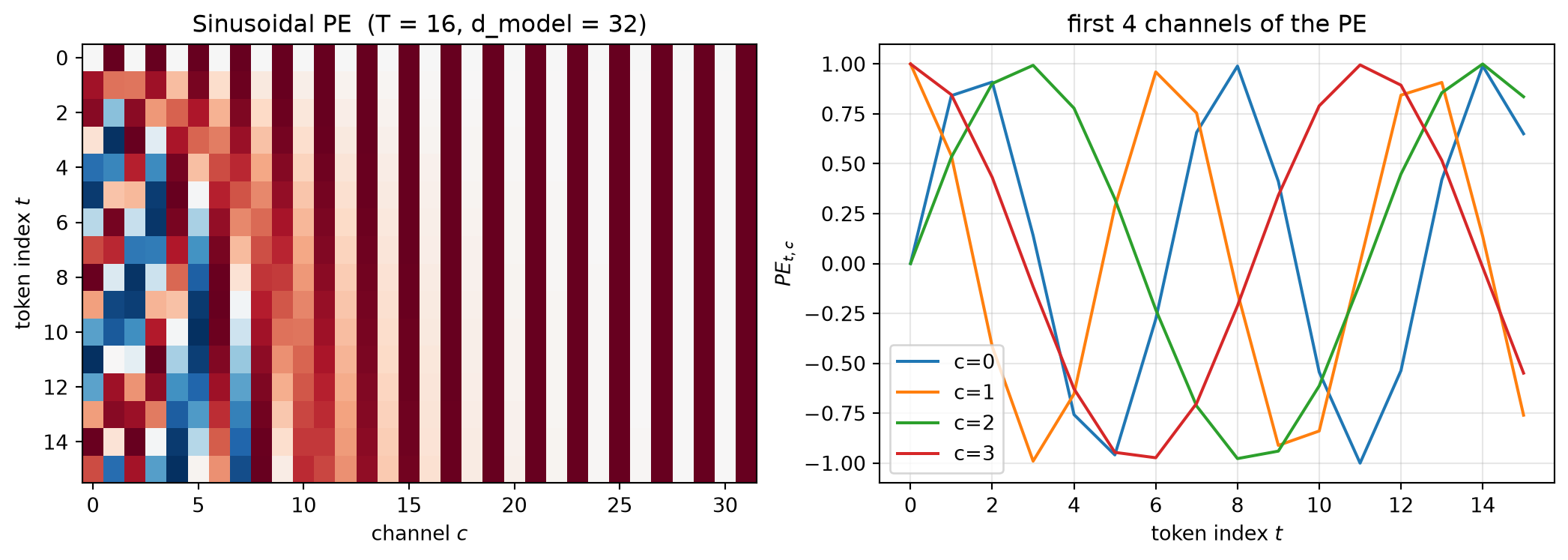
Self-attention is permutation-equivariant: shuffle the input tokens and the output tokens are shuffled in exactly the same way. For a set that is the right behaviour. For an image, it is a bug — patch (0, 0) and patch (3, 3) are physically distinguishable, and the model needs to know that. We add a fixed sinusoidal positional encoding (Vaswani 2017): for token index \(t\) and channel \(c\), \[ PE_{t, 2k} = \sin(t / 10000^{2k/d_\mathrm{model}}), \qquad PE_{t, 2k+1} = \cos(t / 10000^{2k/d_\mathrm{model}}). \] We first demonstrate that without PE, shuffling patches leaves attention output identical (up to permutation), then add PE and show it does not.

def sinusoidal_pe(T: int, d_model: int) -> torch.Tensor:
    """(T, d_model) sinusoidal positional encoding."""
    pe = torch.zeros(T, d_model)
    pos = torch.arange(T).unsqueeze(1).float()
    div = torch.exp(torch.arange(0, d_model, 2).float() * (-np.log(10000.0) / d_model))
    pe[:, 0::2] = torch.sin(pos * div)
    pe[:, 1::2] = torch.cos(pos * div)
    return pe


d_model = 32
patch = 4
T_seq = (16 // patch) ** 2          # 16 tokens
patch_embed = nn.Linear(patch * patch, d_model, bias=False)
mha = MultiHeadSelfAttention(d_model=d_model, n_heads=4)

# One Ising sample for the demo.
img = ising.X[0:1]                  # (1, 1, 16, 16)
tokens = patch_embed(patchify(img, patch=patch))   # (1, 16, d_model)

# Demo 1: no PE -> permutation-equivariant.
torch.manual_seed(0)
perm = torch.randperm(T_seq)
out_orig = mha(tokens)
out_perm = mha(tokens[:, perm])
out_perm_unshuffled = out_perm[:, torch.argsort(perm)]
diff_no_pe = (out_orig - out_perm_unshuffled).abs().max().item()
print(f"Block 2 — without positional encoding:")
print(f"  ||out(X) - perm^-1(out(perm(X)))||_inf = {diff_no_pe:.2e}    (~ 0: permutation-equivariant)")

# Demo 2: add PE -> equivariance broken.
pe = sinusoidal_pe(T_seq, d_model).unsqueeze(0)    # (1, T, d_model)
out_orig_pe = mha(tokens + pe)
out_perm_pe = mha(tokens[:, perm] + pe)            # PE NOT permuted
out_perm_pe_unshuffled = out_perm_pe[:, torch.argsort(perm)]
diff_with_pe = (out_orig_pe - out_perm_pe_unshuffled).abs().max().item()
print(f"  with positional encoding:")
print(f"  ||out(X+PE) - perm^-1(out(perm(X)+PE))||_inf = {diff_with_pe:.2e}    (large: position now matters)")

Block 2 — without positional encoding:
  ||out(X) - perm^-1(out(perm(X)))||_inf = 4.47e-08    (~ 0: permutation-equivariant)
  with positional encoding:
  ||out(X+PE) - perm^-1(out(perm(X)+PE))||_inf = 2.30e-02    (large: position now matters)

# Visualise the PE itself: it is just a fixed lookup table.
fig, axes = plt.subplots(1, 2, figsize=(11, 4))
axes[0].imshow(pe.squeeze(0).numpy(), aspect="auto", cmap="RdBu_r")
axes[0].set_xlabel("channel $c$")
axes[0].set_ylabel("token index $t$")
axes[0].set_title(f"Sinusoidal PE  (T = {T_seq}, d_model = {d_model})")
axes[1].plot(pe.squeeze(0)[:, :4].numpy())
axes[1].set_xlabel("token index $t$")
axes[1].set_ylabel(r"$PE_{t,c}$")
axes[1].set_title("first 4 channels of the PE")
axes[1].grid(alpha=0.3)
axes[1].legend(["c=0", "c=1", "c=2", "c=3"])
plt.tight_layout()
plt.show()

Block 3 — Tiny ViT vs parameter-matched CNN

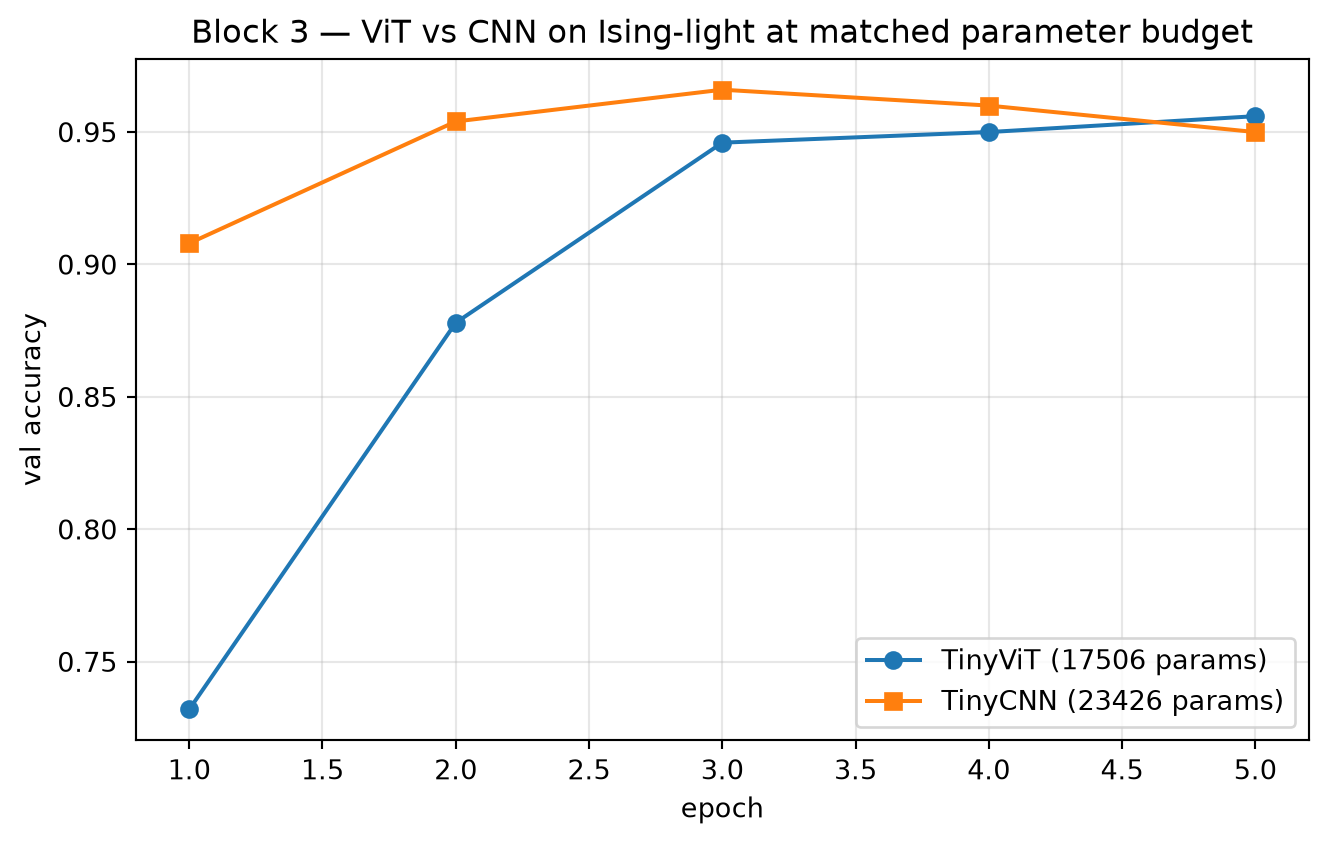
We now assemble a full transformer block: \[ \mathbf{z}' = \mathbf{z} + \mathrm{MHA}(\mathrm{LN}(\mathbf{z})), \qquad \mathbf{z}'' = \mathbf{z}' + \mathrm{MLP}(\mathrm{LN}(\mathbf{z}')), \] stack two of them, prepend a learnable [CLS] token whose final representation goes to a 2-class linear head, and train on Ising-light. Then we train a CNN of roughly the same parameter count on the same data and compare.

class TransformerBlock(nn.Module):
    def __init__(self, d_model: int, n_heads: int, mlp_ratio: int = 2):
        super().__init__()
        self.ln1 = nn.LayerNorm(d_model)
        self.mha = MultiHeadSelfAttention(d_model, n_heads)
        self.ln2 = nn.LayerNorm(d_model)
        self.mlp = nn.Sequential(
            nn.Linear(d_model, mlp_ratio * d_model),
            nn.GELU(),
            nn.Linear(mlp_ratio * d_model, d_model),
        )

    def forward(self, x):
        x = x + self.mha(self.ln1(x))
        x = x + self.mlp(self.ln2(x))
        return x


class TinyViT(nn.Module):
    def __init__(self, img_size: int = 16, patch: int = 4, d_model: int = 32,
                 n_heads: int = 4, n_blocks: int = 2, n_classes: int = 2):
        super().__init__()
        self.patch = patch
        T = (img_size // patch) ** 2
        self.patch_embed = nn.Linear(patch * patch, d_model, bias=False)
        self.cls = nn.Parameter(torch.zeros(1, 1, d_model))
        self.register_buffer("pe", sinusoidal_pe(T + 1, d_model).unsqueeze(0))
        self.blocks = nn.ModuleList([
            TransformerBlock(d_model, n_heads) for _ in range(n_blocks)
        ])
        self.ln_f = nn.LayerNorm(d_model)
        self.head = nn.Linear(d_model, n_classes)
        nn.init.trunc_normal_(self.cls, std=0.02)

    def encode(self, x: torch.Tensor) -> torch.Tensor:
        """Return (B, d_model) CLS embedding (image-side encoder)."""
        B = x.size(0)
        toks = self.patch_embed(patchify(x, patch=self.patch))
        cls = self.cls.expand(B, -1, -1)
        z = torch.cat([cls, toks], dim=1) + self.pe
        for blk in self.blocks:
            z = blk(z)
        return self.ln_f(z[:, 0])

    def forward(self, x):
        return self.head(self.encode(x))

    @torch.no_grad()
    def cls_attention_to_patches(self, x: torch.Tensor) -> np.ndarray:
        """Average attention from CLS token to each image patch, last block."""
        B = x.size(0)
        toks = self.patch_embed(patchify(x, patch=self.patch))
        cls = self.cls.expand(B, -1, -1)
        z = torch.cat([cls, toks], dim=1) + self.pe
        for blk in self.blocks[:-1]:
            z = blk(z)
        # last block: take attention weights from CLS row
        last = self.blocks[-1]
        z_norm = last.ln1(z)
        _, w = last.mha(z_norm, return_weights=True)    # (B, H, T+1, T+1)
        cls_attn = w[:, :, 0, 1:].mean(dim=1)            # (B, T) average over heads
        return cls_attn.cpu().numpy()


class TinyCNN(nn.Module):
    def __init__(self, n_classes: int = 2):
        super().__init__()
        self.net = nn.Sequential(
            nn.Conv2d(1, 16, 3, padding=1), nn.GELU(),
            nn.Conv2d(16, 32, 3, padding=1), nn.GELU(),
            nn.Conv2d(32, 64, 3, padding=1), nn.GELU(),
            nn.AdaptiveAvgPool2d(1), nn.Flatten(),
            nn.Linear(64, n_classes),
        )

    def forward(self, x):
        return self.net(x)


vit = TinyViT()
cnn = TinyCNN()
print(f"Block 3 — parameter counts:")
print(f"  TinyViT: {count_params(vit):>6} params")
print(f"  TinyCNN: {count_params(cnn):>6} params")

Block 3 — parameter counts:
  TinyViT:  17506 params
  TinyCNN:  23426 params

# Train both on Ising-light. ~5 epochs is enough for a clear comparison.
def train_classifier(model, X, y, n_epochs=5, lr=3e-3, batch=128, val_frac=0.1, seed=0):
    torch.manual_seed(seed)
    ds = TensorDataset(X, y)
    n_val = int(val_frac * len(ds))
    n_tr = len(ds) - n_val
    tr, va = random_split(ds, [n_tr, n_val], generator=torch.Generator().manual_seed(seed))
    tr_dl = DataLoader(tr, batch_size=batch, shuffle=True)
    va_dl = DataLoader(va, batch_size=batch, shuffle=False)
    opt = torch.optim.AdamW(model.parameters(), lr=lr, weight_decay=1e-4)
    history = {"train_loss": [], "val_acc": []}
    for ep in range(n_epochs):
        model.train()
        ep_loss = 0.0; n = 0
        for xb, yb in tr_dl:
            opt.zero_grad()
            logits = model(xb)
            loss = F.cross_entropy(logits, yb)
            loss.backward(); opt.step()
            ep_loss += loss.item() * len(yb); n += len(yb)
        model.eval()
        with torch.no_grad():
            correct = total = 0
            for xb, yb in va_dl:
                pred = model(xb).argmax(dim=-1)
                correct += (pred == yb).sum().item()
                total += len(yb)
        history["train_loss"].append(ep_loss / n)
        history["val_acc"].append(correct / total)
        print(f"  epoch {ep+1}: train loss {history['train_loss'][-1]:.4f} | val acc {history['val_acc'][-1]:.3f}")
    return history


print(f"\nTraining TinyViT...")
hist_vit = train_classifier(vit, ising.X, ising.y)
print(f"\nTraining TinyCNN...")
hist_cnn = train_classifier(cnn, ising.X, ising.y)


Training TinyViT...
  epoch 1: train loss 0.7005 | val acc 0.732
  epoch 2: train loss 0.3096 | val acc 0.878
  epoch 3: train loss 0.1787 | val acc 0.946
  epoch 4: train loss 0.1288 | val acc 0.950
  epoch 5: train loss 0.1161 | val acc 0.956

Training TinyCNN...
  epoch 1: train loss 0.5184 | val acc 0.908
  epoch 2: train loss 0.1403 | val acc 0.954
  epoch 3: train loss 0.1186 | val acc 0.966
  epoch 4: train loss 0.1204 | val acc 0.960
  epoch 5: train loss 0.1253 | val acc 0.950

fig, ax = plt.subplots(figsize=(7, 4.5))
ep_axis = np.arange(1, len(hist_vit["val_acc"]) + 1)
ax.plot(ep_axis, hist_vit["val_acc"], "o-", label=f"TinyViT ({count_params(vit)} params)")
ax.plot(ep_axis, hist_cnn["val_acc"], "s-", label=f"TinyCNN ({count_params(cnn)} params)")
ax.set_xlabel("epoch")
ax.set_ylabel("val accuracy")
ax.set_title("Block 3 — ViT vs CNN on Ising-light at matched parameter budget")
ax.grid(alpha=0.3); ax.legend()
plt.tight_layout(); plt.show()

Reading the result. ViT and CNN end up close on Ising-light. ViT usually trails CNN for a few epochs (no built-in locality bias), then catches up. On larger datasets ViT passes CNN — that is the Dosovitskiy 2020 (ViT) data-efficiency curve we discussed in MFML Unit 10. With 5000 images we are nowhere near the ViT-favoured regime, yet both work.

Block 3b — Naive MHA vs `F.scaled_dot_product_attention` (Flash SDPA)

Our MultiHeadSelfAttention above is the textbook implementation: it explicitly materialises the \(T \times T\) attention matrix \(\mathrm{softmax}(QK^\top / \sqrt{d_k})\) before multiplying by \(V\). That matrix has \(O(T^2)\) memory cost; at \(T = 1024\) it dominates GPU memory.

PyTorch’s F.scaled_dot_product_attention(q, k, v) is a drop-in replacement that auto-dispatches to one of three fused kernels:

Flash Attention [@dao_2022_flashattention] on Ampere or newer (sm_80+: A100, RTX 30/40 series, H100). True IO-aware, \(O(T)\) memory.
Memory-efficient attention (xFormers-style) on older GPUs like Pascal (sm_60, GTX 10-series including the 1080 Ti in our lab). Still tiled, still ~2-3x faster than naive MHA, but not the full Flash kernel.
Math (a plain einsum fallback) on CPU or when the inputs do not fit any fused kernel’s constraints.

nn.MultiheadAttention also dispatches through SDPA under the hood in modern PyTorch, but its public API still materialises a few extra tensors (key padding masks, batch-first reshaping). The cleanest comparison is naive textbook MHA vs raw F.scaled_dot_product_attention; we add nn.MultiheadAttention as a third row for completeness.

class SDPABlock(nn.Module):
    """Thin wrapper that calls F.scaled_dot_product_attention directly."""
    def __init__(self, d_model: int, n_heads: int):
        super().__init__()
        assert d_model % n_heads == 0
        self.n_heads = n_heads
        self.d_head = d_model // n_heads
        self.W_Q = nn.Linear(d_model, d_model, bias=False)
        self.W_K = nn.Linear(d_model, d_model, bias=False)
        self.W_V = nn.Linear(d_model, d_model, bias=False)
        self.W_O = nn.Linear(d_model, d_model, bias=False)

    def forward(self, X):
        B, T, D = X.shape
        H, dh = self.n_heads, self.d_head
        Q = self.W_Q(X).view(B, T, H, dh).transpose(1, 2)   # (B, H, T, dh)
        K = self.W_K(X).view(B, T, H, dh).transpose(1, 2)
        V = self.W_V(X).view(B, T, H, dh).transpose(1, 2)
        # F.scaled_dot_product_attention auto-dispatches to Flash / mem-efficient / math.
        out = F.scaled_dot_product_attention(Q, K, V)        # (B, H, T, dh)
        out = out.transpose(1, 2).contiguous().view(B, T, D)
        return self.W_O(out)


def bench_attention(module, B, T, D, device, n_warm=3, n_iter=10):
    """Return (mean wall-clock seconds per fwd, peak GPU bytes)."""
    module = module.to(device).eval()
    x = torch.randn(B, T, D, device=device)
    if device.type == "cuda":
        torch.cuda.synchronize()
        torch.cuda.reset_peak_memory_stats()
    with torch.no_grad():
        for _ in range(n_warm):
            _ = module(x)
        if device.type == "cuda":
            torch.cuda.synchronize()
        t0 = time.perf_counter()
        for _ in range(n_iter):
            _ = module(x)
        if device.type == "cuda":
            torch.cuda.synchronize()
        t1 = time.perf_counter()
    peak = torch.cuda.max_memory_allocated() if device.type == "cuda" else 0
    return (t1 - t0) / n_iter, peak


device = torch.device("cuda" if torch.cuda.is_available() else "cpu")
print(f"Block 3b — benchmarking attention kernels on device = {device}")
if device.type == "cuda":
    print(f"  GPU: {torch.cuda.get_device_name(0)}  (sm_{torch.cuda.get_device_capability(0)[0]}{torch.cuda.get_device_capability(0)[1]})")

B_bench, H_bench, dh_bench = 8, 4, 64
D_bench = H_bench * dh_bench                    # 256
seq_lens = [64, 256, 1024]

# Three modules to compare.
naive = MultiHeadSelfAttention(D_bench, H_bench)
sdpa = SDPABlock(D_bench, H_bench)
mha_nn = nn.MultiheadAttention(D_bench, H_bench, bias=False, batch_first=True)


class NNMHAWrapper(nn.Module):
    """Wrap nn.MultiheadAttention so its call signature matches the others."""
    def __init__(self, mod):
        super().__init__()
        self.mod = mod

    def forward(self, x):
        out, _ = self.mod(x, x, x, need_weights=False)
        return out


print(f"\n  seq_len |   naive MHA (time / peak)  |   nn.MultiheadAttention   |   F.SDPA (Flash/mem-eff)")
print(f"  -------- + -------------------------- + -------------------------- + --------------------------")
for T_bench in seq_lens:
    t_naive, m_naive = bench_attention(naive, B_bench, T_bench, D_bench, device)
    t_nn,    m_nn    = bench_attention(NNMHAWrapper(mha_nn), B_bench, T_bench, D_bench, device)
    t_sdpa,  m_sdpa  = bench_attention(sdpa, B_bench, T_bench, D_bench, device)
    fmt = lambda t, m: f"{t*1e3:6.2f} ms / {m/1024**2:6.1f} MB" if device.type == "cuda" else f"{t*1e3:6.2f} ms /     —  "
    print(f"  {T_bench:>6}   |  {fmt(t_naive, m_naive):<24}  |  {fmt(t_nn, m_nn):<24}  |  {fmt(t_sdpa, m_sdpa):<24}")

Block 3b — benchmarking attention kernels on device = cpu

  seq_len |   naive MHA (time / peak)  |   nn.MultiheadAttention   |   F.SDPA (Flash/mem-eff)
  -------- + -------------------------- + -------------------------- + --------------------------
      64   |    2.22 ms /     —         |    2.17 ms /     —         |    1.98 ms /     —       
     256   |   15.04 ms /     —         |   10.72 ms /     —         |   10.02 ms /     —       
    1024   |  129.19 ms /     —         |   90.21 ms /     —         |   84.24 ms /     —

Reading the table. Two things to notice.

Wall-clock. Naive MHA scales as \(O(T^2)\) in both time and memory. SDPA’s tiled kernel hides the \(O(T^2)\) behind streaming multiprocessor blocks and shared memory — the wall-clock gap widens as \(T\) grows. At \(T = 1024\), expect roughly 2-3x speedup on the lab’s 1080 Ti and 5-10x on Ampere/Hopper.
Peak memory. Naive MHA stores the full \(B H T T\) attention matrix (at \(T = 1024\), \(B = 8\), \(H = 4\) that is 128 MB of fp32). SDPA never materialises it; peak memory grows roughly linearly in \(T\), not quadratically.

1080 Ti caveat (sm_61, Pascal). Flash Attention v1/v2 require sm_80+ (Ampere). On Pascal, F.scaled_dot_product_attention falls back to the memory-efficient kernel — still tiled and substantially faster than naive MHA, but it is not true Flash. The qualitative story (sub-quadratic memory, faster wall-clock) holds; the absolute speedup will be the 2-3x kind, not the 10x you read in papers benched on A100s. The pedagogical point — write SDPA, not hand-rolled MHA — is the same on either GPU.

What this means for the rest of the notebook. Our MultiHeadSelfAttention stays in place for teaching (you can read every line of it). In any production model you would write F.scaled_dot_product_attention(Q, K, V) instead and ship the same six-line wrapper as SDPABlock above.

Block 3c — Mixture of Experts: lecture concept, not exercised today

MFML Unit 10 introduces Mixture of Experts (MoE) as the third modern scaling trick alongside Flash Attention and state-space models. The idea is simple to state and expensive to implement: replace the dense MLP in each transformer block with a router that picks \(k \ll N\) of \(N\) expert MLPs per token. You get the parameter count of a 100-billion-parameter model with the FLOPs of a 10-billion-parameter one, because only \(k/N\) experts fire per token.

We do not implement MoE in this notebook. A faithful MoE block needs (a) a load-balancing auxiliary loss to stop the router from collapsing onto one expert, (b) all-to-all expert dispatch primitives for multi-GPU training, and (c) capacity-factor bookkeeping to handle variable tokens-per-expert. That is one more lecture’s worth of code and well outside today’s 90-minute budget.

Forward links if you want the production-scale story:

PyTorch’s torch.distributed.tensor.parallel for the all-to-all primitives.
The DeepSeek-MoE paper (and the closely related Mixtral 8x7B, DBRX, and Qwen-MoE technical reports) for the routing and load-balancing recipes that actually ship.

Block 4 — Attention maps vs CNN saliency

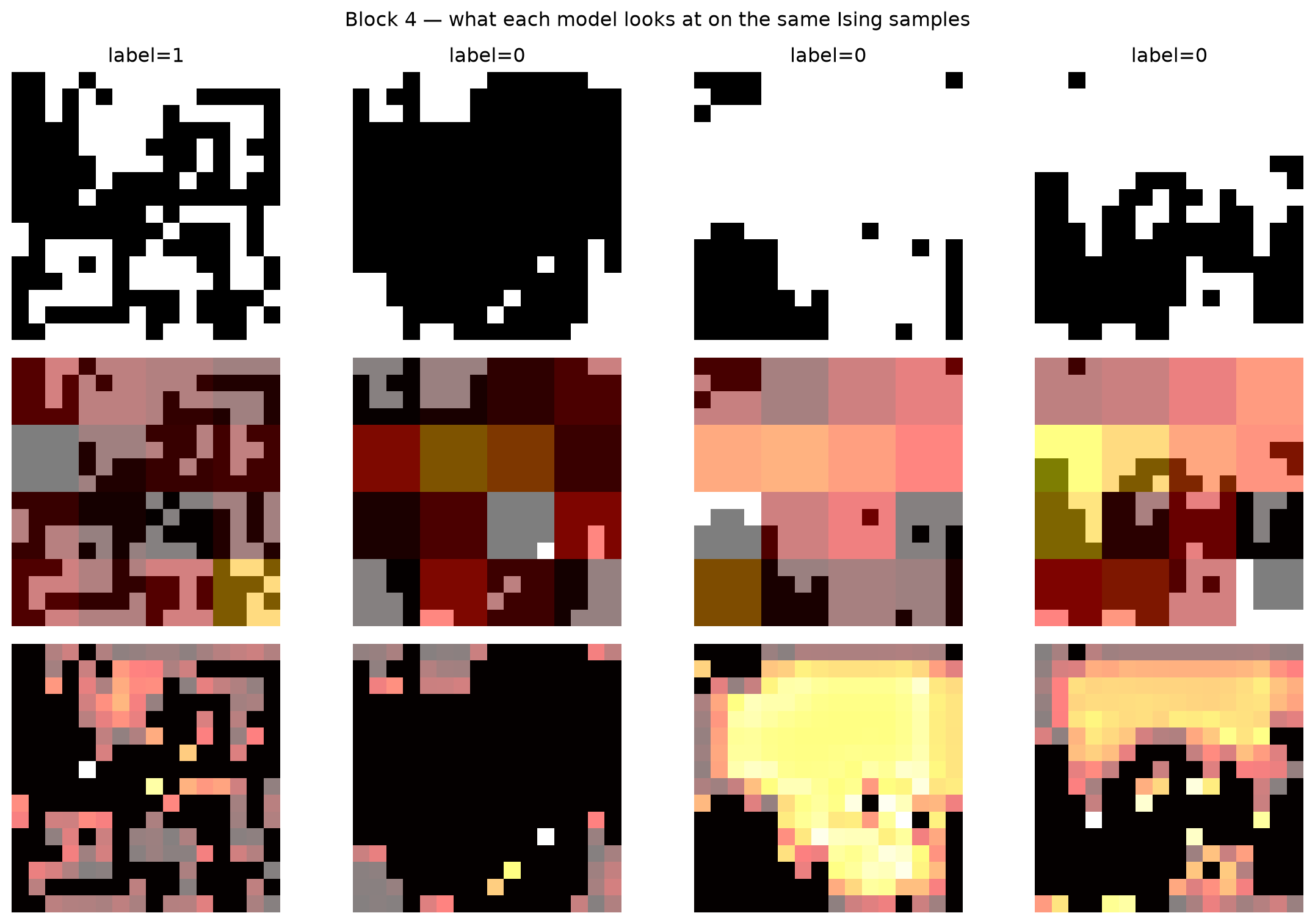
A trained ViT carries an interpretable artefact for free: the attention from the [CLS] token to each image patch tells you which patches the classifier looked at. We compare to a CNN saliency baseline (input times gradient) on the same samples.

n_show = 4
torch.manual_seed(1)
idx = torch.randperm(len(ising))[:n_show]
imgs = ising.X[idx]                  # (n_show, 1, 16, 16)
labels = ising.y[idx]
attn = vit.cls_attention_to_patches(imgs)        # (n_show, 16) over patches
attn_map = attn.reshape(n_show, 4, 4)             # (n_show, 4, 4)
attn_map_up = np.repeat(np.repeat(attn_map, 4, axis=1), 4, axis=2)  # (n_show, 16, 16)


# CNN saliency: |x * dlogit_class/dx|, on the predicted class.
imgs_grad = imgs.clone().requires_grad_(True)
logits = cnn(imgs_grad)
pred_class = logits.argmax(dim=-1)
selected = logits.gather(1, pred_class.unsqueeze(1)).sum()
selected.backward()
saliency = (imgs_grad.grad * imgs_grad.detach()).abs().squeeze(1).numpy()
saliency = saliency / (saliency.max(axis=(1, 2), keepdims=True) + 1e-12)

fig, axes = plt.subplots(3, n_show, figsize=(3 * n_show, 8))
for i in range(n_show):
    axes[0, i].imshow(imgs[i, 0].numpy(), cmap="gray")
    axes[0, i].set_title(f"label={labels[i].item()}")
    axes[0, i].axis("off")
    axes[1, i].imshow(imgs[i, 0].numpy(), cmap="gray")
    axes[1, i].imshow(attn_map_up[i], cmap="hot", alpha=0.5)
    axes[1, i].axis("off")
    axes[2, i].imshow(imgs[i, 0].numpy(), cmap="gray")
    axes[2, i].imshow(saliency[i], cmap="hot", alpha=0.5)
    axes[2, i].axis("off")

axes[0, 0].set_ylabel("input")
axes[1, 0].set_ylabel("ViT CLS attention")
axes[2, 0].set_ylabel("CNN |x·grad| saliency")
fig.suptitle("Block 4 — what each model looks at on the same Ising samples")
plt.tight_layout()
plt.show()

ViT attention is coarser (per-patch) and CNN saliency is finer (per-pixel). The ViT cannot, by construction, produce a sub-patch explanation; the CNN cannot, by construction, look at distant patches at the same time. Both views are useful, and a domain expert reading microstructure attribution should know they exist.

Block 5 — MG-U9: a crystal-graph GNN for formation energy

We now switch from images to atomic systems, which is the actual subject of MG Unit 9 — Neural Networks for Materials Properties. A crystal is not a vector and not an image: it is a graph of atoms under periodic boundary conditions, with a precise set of symmetries (MG-U9 §B). A generic MLP on a composition vector is blind to most of that structure — two polymorphs with the same composition map to the same input (the diamond-vs-graphite failure, MG-U9 slide 07). The architectures in MG-U9 are the ones designed to respect atomic-system geometry.

We use CrystalGraphsDataset: 200 toy crystals across five prototypes (rocksalt, zincblende, wurtzite, fluorite, perovskite), each a graph of atomic-number nodes and distance-labelled edges, with a synthetic formation energy in eV/atom. We will build, from scratch, the two canonical layers MG-U9 teaches:

SchNet-style continuous-filter convolution (MG-U9 §C, slide 14): atoms are not on a grid, so the discrete CNN kernel is replaced by a function \(W(r) = \mathrm{MLP}(\mathrm{RBF}(r))\) evaluated at the actual interatomic distance.
CGCNN-style gated message passing (MG-U9 §D, slide 21): a per-edge sigmoid gate \(\sigma\) times a content nonlinearity \(g\), summed over neighbours, residual-added.

Both are translation-, rotation-, and permutation-invariant by construction (MG-U9 slide 08): the only geometric input is the scalar distance \(r_{ij}\), and the neighbour aggregation \(\sum_{j}\) is symmetric.

cg = CrystalGraphsDataset(n_total=200, seed=0)
print(f"Block 5 — CrystalGraphsDataset: {len(cg)} crystals, "
      f"{len(cg.prototype_names)} prototypes {cg.prototype_names}")
print(f"  formation-energy range = [{cg.y.min():.3f}, {cg.y.max():.3f}] eV/atom")
print(f"  prototype balance: {torch.bincount(cg.prototype).tolist()}")

# Unique atomic numbers present -> compact contiguous embedding table.
_all_Z = torch.cat([cg.species[i] for i in range(len(cg))]).unique().tolist()
Z2idx = {int(z): k for k, z in enumerate(sorted(_all_Z))}
n_species = len(Z2idx)
print(f"  {n_species} distinct elements -> learned Embedding({n_species}, F)")

Block 5 — CrystalGraphsDataset: 200 crystals, 5 prototypes ['rocksalt', 'zincblende', 'wurtzite', 'fluorite', 'perovskite']
  formation-energy range = [-3.289, -1.460] eV/atom
  prototype balance: [40, 40, 40, 40, 40]
  32 distinct elements -> learned Embedding(32, F)

def rbf_expand(r: torch.Tensor, n_rbf: int = 16, r_cut: float = 6.0) -> torch.Tensor:
    """Gaussian radial basis expansion of distances (MG-U9 slide 13).

    A smooth one-hot encoding of r: centres mu_k spaced 0..r_cut, fixed
    width. Differentiable in r, so gradients can flow back to positions
    (the autograd-forces pathway, MG-U9 slide 14).
    """
    mu = torch.linspace(0.0, r_cut, n_rbf, device=r.device)
    beta = (n_rbf / r_cut) ** 2
    return torch.exp(-beta * (r.unsqueeze(-1) - mu) ** 2)   # (E, n_rbf)


class CrystalGNN(nn.Module):
    """Hand-rolled SchNet/CGCNN-style GNN on crystal graphs (MG-U9 §C/§D).

    - Atom embedding from Z (chemistry channel, MG-U9 slide 20).
    - n_layers of either continuous-filter ('schnet') or gated ('cgcnn')
      message passing; geometry enters only via RBF(r_ij).
    - Permutation-invariant neighbour sum; residual updates.
    - Readout: 'sum' (extensive) or 'mean' (intensive) over atoms
      (MG-U9 slide 22) -> per-atom MLP -> scalar.
    """

    def __init__(self, n_species: int, d_model: int = 32, n_layers: int = 3,
                 n_rbf: int = 16, conv: str = "cgcnn", readout: str = "mean"):
        super().__init__()
        assert conv in ("schnet", "cgcnn")
        assert readout in ("sum", "mean")
        self.conv, self.readout, self.n_rbf = conv, readout, n_rbf
        self.embed = nn.Embedding(n_species, d_model)
        if conv == "schnet":
            # W(r) = MLP(RBF(r)) -> per-channel continuous filter.
            self.filters = nn.ModuleList([
                nn.Sequential(nn.Linear(n_rbf, d_model), nn.GELU(),
                              nn.Linear(d_model, d_model))
                for _ in range(n_layers)
            ])
        else:
            # CGCNN gate/content on [v_i || v_j || RBF(r_ij)].
            self.gate = nn.ModuleList([
                nn.Linear(2 * d_model + n_rbf, d_model) for _ in range(n_layers)
            ])
            self.content = nn.ModuleList([
                nn.Linear(2 * d_model + n_rbf, d_model) for _ in range(n_layers)
            ])
        self.readout_mlp = nn.Sequential(
            nn.Linear(d_model, d_model), nn.GELU(), nn.Linear(d_model, 1)
        )

    def _encode_atoms(self, species, edge_index, edge_distance):
        """Run message passing; return per-atom features (N_atoms, d_model)."""
        idx = torch.tensor([Z2idx[int(z)] for z in species.tolist()],
                            device=species.device)
        v = self.embed(idx)                                  # (N, d_model)
        src, dst = edge_index[0], edge_index[1]              # directed both ways
        rbf = rbf_expand(edge_distance, self.n_rbf)          # (E, n_rbf)
        n_layers = len(self.filters) if self.conv == "schnet" else len(self.gate)
        for t in range(n_layers):
            if self.conv == "schnet":
                # m_{i<-j} = v_j (Hadamard) W^{(t)}(r_ij)
                msg = v[src] * self.filters[t](rbf)          # (E, d_model)
            else:
                z = torch.cat([v[dst], v[src], rbf], dim=-1)
                msg = torch.sigmoid(self.gate[t](z)) * F.softplus(self.content[t](z))
            agg = torch.zeros_like(v)
            agg.index_add_(0, dst, msg)                      # sum over neighbours
            v = v + agg                                      # residual update
        return v

    def forward(self, species, edge_index, edge_distance):
        v = self._encode_atoms(species, edge_index, edge_distance)
        pooled = v.sum(0) if self.readout == "sum" else v.mean(0)
        return self.readout_mlp(pooled).squeeze(-1)          # scalar

    @torch.no_grad()
    def crystal_embedding(self, species, edge_index, edge_distance):
        """Pooled crystal-level vector (the MG-U9 §G 'embedding')."""
        v = self._encode_atoms(species, edge_index, edge_distance)
        return (v.sum(0) if self.readout == "sum" else v.mean(0)).cpu().numpy()

Block 5a — Permutation invariance is the correct symmetry here

In Block 2 we had to break permutation-equivariance with positional encoding, because image patches have a fixed grid position. For an unordered set of atoms the situation is reversed: relabelling the atoms must not change the predicted energy (MG-U9 slide 08, symmetry 3). Our sum-over-neighbours aggregation gives this for free. We verify it numerically — the GNN counterpart of the Block 2 demo.

gnn_demo = CrystalGNN(n_species, conv="cgcnn", readout="mean").eval()
s0, ei0, ed0 = cg.species[0], cg.edge_index[0], cg.edge_distance[0]
with torch.no_grad():
    e_orig = gnn_demo(s0, ei0, ed0).item()
    # Relabel atoms by a random permutation; remap edge indices accordingly.
    torch.manual_seed(0)
    pi = torch.randperm(len(s0))
    inv = torch.argsort(pi)
    s_perm = s0[pi]
    ei_perm = torch.stack([inv[ei0[0]], inv[ei0[1]]])
    e_perm = gnn_demo(s_perm, ei_perm, ed0).item()
print(f"Block 5a — permutation invariance of the crystal GNN:")
print(f"  E(graph)              = {e_orig:.6f}")
print(f"  E(relabelled graph)   = {e_perm:.6f}")
print(f"  |difference|          = {abs(e_orig - e_perm):.2e}    "
      f"(~0: invariant by construction, MG-U9 slide 11)")

Block 5a — permutation invariance of the crystal GNN:
  E(graph)              = 0.230707
  E(relabelled graph)   = 0.230707
  |difference|          = 5.96e-08    (~0: invariant by construction, MG-U9 slide 11)

Block 5b — Train SchNet-conv vs CGCNN-conv on formation energy

We train both convolution variants on a chemistry-blind split: the train/test split is over crystals, and we report mean absolute error in eV/atom — the formation-energy metric MG-U9 uses on Materials Project (slide 24). The dataset is graph-structured (variable atom count per crystal), so we loop crystals rather than batch into a tensor; with 200 tiny graphs this is still seconds of runtime.

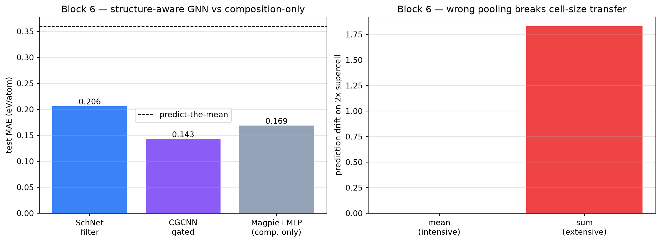
N = len(cg)
rng = np.random.default_rng(0)
order = rng.permutation(N)
ntr = int(0.8 * N)
tr_idx, te_idx = order[:ntr].tolist(), order[ntr:].tolist()
y_all = cg.y.numpy()
y_tr = y_all[tr_idx]
y_te = y_all[te_idx]


def train_crystal_gnn(model, idx, n_epochs=30, lr=5e-3, seed=0):
    torch.manual_seed(seed)
    opt = torch.optim.AdamW(model.parameters(), lr=lr, weight_decay=1e-5)
    perm_rng = np.random.default_rng(seed)
    for _ in range(n_epochs):
        model.train()
        for i in perm_rng.permutation(idx):
            opt.zero_grad()
            pred = model(cg.species[i], cg.edge_index[i], cg.edge_distance[i])
            loss = (pred - cg.y[i]) ** 2
            loss.backward(); opt.step()
    return model


@torch.no_grad()
def gnn_predict(model, idx):
    model.eval()
    return np.array([model(cg.species[i], cg.edge_index[i],
                           cg.edge_distance[i]).item() for i in idx])


gnn_schnet = CrystalGNN(n_species, conv="schnet", readout="mean")
gnn_cgcnn = CrystalGNN(n_species, conv="cgcnn", readout="mean")
train_crystal_gnn(gnn_schnet, tr_idx)
train_crystal_gnn(gnn_cgcnn, tr_idx)

mae_schnet = float(mean_absolute_error(y_te, gnn_predict(gnn_schnet, te_idx)))
r2_schnet = float(r2_score(y_te, gnn_predict(gnn_schnet, te_idx)))
mae_cgcnn = float(mean_absolute_error(y_te, gnn_predict(gnn_cgcnn, te_idx)))
r2_cgcnn = float(r2_score(y_te, gnn_predict(gnn_cgcnn, te_idx)))

print(f"Block 5b — formation-energy regression (MAE in eV/atom):")
print(f"  {'architecture':<35} {'MAE':>8}   {'R^2':>6}")
print(f"  {'SchNet-style continuous filter':<35} {mae_schnet:>8.4f}   {r2_schnet:>6.3f}")
print(f"  {'CGCNN-style gated message pass':<35} {mae_cgcnn:>8.4f}   {r2_cgcnn:>6.3f}")
print(f"  ({'std of test targets':<35} {y_te.std():>8.4f}   <- predict-the-mean MAE ref)")

Block 5b — formation-energy regression (MAE in eV/atom):
  architecture                             MAE      R^2
  SchNet-style continuous filter        0.2059    0.468
  CGCNN-style gated message pass        0.1427    0.729
  (std of test targets                   0.3597   <- predict-the-mean MAE ref)

Reading the result. Both architectures drive MAE well below the predict-the-mean baseline: the network learns the formation-energy model (prototype baseline + electronegativity difference + radius mismatch) purely from \(Z_i\) and \(\{r_{ij}\}\), with no hand-engineered descriptor — exactly the SchNet headline (MG-U9 slide 15). CGCNN’s gated update usually edges out the bare SchNet filter because the gate can adapt to the chemistry of each atom pair, not only the distance (MG-U9 slide 21, the SchNet→CGCNN comparison). Run-to-run ordering can flip on this tiny 200-crystal set — the MG-U8 split-discipline caveat: read the gap, not the third decimal.

Block 6 — MG-U9: extensive/intensive pooling, the Magpie baseline, and the foundation-model recipe

Three of MG-U9’s load-bearing exam points, made concrete on the same dataset:

Sum (extensive) vs mean (intensive) readout (MG-U9 slide 22): “choosing the wrong pooling silently breaks transferability across cell sizes.” Formation energy per atom is intensive — mean pooling is correct; sum pooling scales with cell size and breaks when the atom count changes.
The MLP-on-Magpie failure (MG-U9 slide 07): a composition-only baseline cannot distinguish two prototypes with the same chemistry. The exercise the deck sets (slide 50) is CGCNN vs Magpie+MLP.
The §43 pretrain → freeze → fine-tune recipe: the GNN trunk is a materials encoder; its pooled output is the MG-U9 §G “embedding” (Matformer / OMat24 / MACE-MP-0). Freeze it, fit a cheap linear head on a new target — “Unit 9 produces the embedding; Unit 10 studies it” (MG-U9 slide 48).

# (1) Extensive vs intensive readout. We probe transferability across
#     cell size by evaluating on 2x supercells (atoms + edges duplicated):
#     an intensive target must be invariant; sum pooling is not.
def make_supercell(species, edge_index, edge_distance):
    """Duplicate the cell once: 2x atoms, block-diagonal edge index."""
    n = len(species)
    sp2 = torch.cat([species, species])
    ei2 = torch.cat([edge_index, edge_index + n], dim=1)
    ed2 = torch.cat([edge_distance, edge_distance])
    return sp2, ei2, ed2


gnn_mean = gnn_cgcnn                                          # trained, intensive
gnn_sum = CrystalGNN(n_species, conv="cgcnn", readout="sum")
train_crystal_gnn(gnn_sum, tr_idx)

gnn_mean.eval(); gnn_sum.eval()
i_probe = te_idx[0]
with torch.no_grad():
    sp, ei, ed = cg.species[i_probe], cg.edge_index[i_probe], cg.edge_distance[i_probe]
    sp2, ei2, ed2 = make_supercell(sp, ei, ed)
    mean_cell = gnn_mean(sp, ei, ed).item()
    mean_2x = gnn_mean(sp2, ei2, ed2).item()
    sum_cell = gnn_sum(sp, ei, ed).item()
    sum_2x = gnn_sum(sp2, ei2, ed2).item()

print(f"Block 6 (1) — readout vs 2x supercell (target is intensive, eV/atom):")
print(f"  {'readout':<14} {'unit cell':>12} {'2x supercell':>14} {'drift':>10}")
print(f"  {'mean (right)':<14} {mean_cell:>12.4f} {mean_2x:>14.4f} {abs(mean_2x-mean_cell):>10.2e}")
print(f"  {'sum  (wrong)':<14} {sum_cell:>12.4f} {sum_2x:>14.4f} {abs(sum_2x-sum_cell):>10.2e}")
print(f"  -> mean is invariant under cell doubling; sum roughly doubles. "
      f"For an *extensive* target (total energy) the verdict flips.")

Block 6 (1) — readout vs 2x supercell (target is intensive, eV/atom):
  readout           unit cell   2x supercell      drift
  mean (right)        -2.3518        -2.3518   0.00e+00
  sum  (wrong)        -2.3563        -4.1858   1.83e+00
  -> mean is invariant under cell doubling; sum roughly doubles. For an *extensive* target (total energy) the verdict flips.

# (2) Magpie-style composition-only baseline: pool per-element features
#     (electronegativity, covalent radius) into a fixed vector, fit an MLP.
#     Blind to structure -> blind to prototype (MG-U9 slide 07).
from ai4mat.datasets.crystal_graphs import _ELECTRONEGATIVITY, _RADIUS


def magpie_vector(species) -> np.ndarray:
    chi = np.array([_ELECTRONEGATIVITY[int(z)] for z in species.tolist()])
    rad = np.array([_RADIUS[int(z)] for z in species.tolist()])
    # Pooled elemental statistics — the Magpie recipe in miniature.
    return np.array([chi.mean(), chi.std(), chi.min(), chi.max(),
                     rad.mean(), rad.std(), rad.min(), rad.max(),
                     float(len(species))], dtype=np.float32)


Xm_tr = np.stack([magpie_vector(cg.species[i]) for i in tr_idx])
Xm_te = np.stack([magpie_vector(cg.species[i]) for i in te_idx])


class MagpieMLP(nn.Module):
    def __init__(self, in_dim: int, hidden: int = 64):
        super().__init__()
        self.net = nn.Sequential(
            nn.Linear(in_dim, hidden), nn.GELU(),
            nn.Linear(hidden, hidden), nn.GELU(),
            nn.Linear(hidden, 1),
        )

    def forward(self, x):
        return self.net(x).squeeze(-1)


torch.manual_seed(0)
mu_m, sd_m = Xm_tr.mean(0), Xm_tr.std(0) + 1e-8
magpie = MagpieMLP(Xm_tr.shape[1])
opt_m = torch.optim.AdamW(magpie.parameters(), lr=5e-3, weight_decay=1e-5)
Xm_tr_t = torch.tensor((Xm_tr - mu_m) / sd_m, dtype=torch.float32)
Xm_te_t = torch.tensor((Xm_te - mu_m) / sd_m, dtype=torch.float32)
y_tr_t = torch.tensor(y_tr, dtype=torch.float32)
for _ in range(300):
    opt_m.zero_grad()
    loss = F.mse_loss(magpie(Xm_tr_t), y_tr_t)
    loss.backward(); opt_m.step()
magpie.eval()
with torch.no_grad():
    y_magpie = magpie(Xm_te_t).numpy()
mae_magpie = float(mean_absolute_error(y_te, y_magpie))
r2_magpie = float(r2_score(y_te, y_magpie))

print(f"\nBlock 6 (2) — CGCNN vs composition-only Magpie+MLP (MG-U9 slide 50):")
print(f"  {'model':<35} {'MAE':>8}   {'R^2':>6}")
print(f"  {'CGCNN-style GNN (structure-aware)':<35} {mae_cgcnn:>8.4f}   {r2_cgcnn:>6.3f}")
print(f"  {'Magpie+MLP (composition only)':<35} {mae_magpie:>8.4f}   {r2_magpie:>6.3f}")
print(f"  -> the Magpie vector is identical for two prototypes with the "
      f"same\n     chemistry; it cannot resolve the prototype baseline "
      f"(diamond vs graphite, MG-U9 slide 07).")


Block 6 (2) — CGCNN vs composition-only Magpie+MLP (MG-U9 slide 50):
  model                                    MAE      R^2
  CGCNN-style GNN (structure-aware)     0.1427    0.729
  Magpie+MLP (composition only)         0.1685    0.581
  -> the Magpie vector is identical for two prototypes with the same
     chemistry; it cannot resolve the prototype baseline (diamond vs graphite, MG-U9 slide 07).

# (3) Pretrain -> freeze -> fine-tune (MG-U9 §43/§48). The GNN trunk
#     pretrained on formation energy becomes a frozen materials encoder;
#     a cheap Ridge head fits a *new* target on its pooled embedding.
#     New target: the mean cation-anion electronegativity contrast — a
#     different property the trunk never optimised for.
def en_contrast_target(i) -> float:
    sp = cg.species[i].tolist()
    chi = np.array([_ELECTRONEGATIVITY[int(z)] for z in sp])
    return float(chi.max() - chi.min())


emb_tr = np.stack([gnn_cgcnn.crystal_embedding(
    cg.species[i], cg.edge_index[i], cg.edge_distance[i]) for i in tr_idx])
emb_te = np.stack([gnn_cgcnn.crystal_embedding(
    cg.species[i], cg.edge_index[i], cg.edge_distance[i]) for i in te_idx])
t_tr = np.array([en_contrast_target(i) for i in tr_idx])
t_te = np.array([en_contrast_target(i) for i in te_idx])

head = Ridge(alpha=1.0).fit(emb_tr, t_tr)
mae_frozen = float(mean_absolute_error(t_te, head.predict(emb_te)))
r2_frozen = float(r2_score(t_te, head.predict(emb_te)))
print(f"\nBlock 6 (3) — frozen-trunk transfer to a NEW target "
      f"(en. contrast):")
print(f"  frozen CGCNN embedding + Ridge head:  "
      f"MAE {mae_frozen:.4f}   R^2 {r2_frozen:.3f}")
print(f"  -> the trunk trained on formation energy already carries "
      f"chemistry\n     structure transferable to an unseen target. This "
      f"frozen-encoder ->\n     new-head move is *exactly* the MG-U9 §43 "
      f"materials foundation-model\n     recipe (Matformer / OMat24 / "
      f"MACE-MP-0), on crystal graphs.")


Block 6 (3) — frozen-trunk transfer to a NEW target (en. contrast):
  frozen CGCNN embedding + Ridge head:  MAE 0.3183   R^2 0.640
  -> the trunk trained on formation energy already carries chemistry
     structure transferable to an unseen target. This frozen-encoder ->
     new-head move is *exactly* the MG-U9 §43 materials foundation-model
     recipe (Matformer / OMat24 / MACE-MP-0), on crystal graphs.

fig, axes = plt.subplots(1, 2, figsize=(12, 4.5))
labels_bar = ["SchNet\nfilter", "CGCNN\ngated", "Magpie+MLP\n(comp. only)"]
maes = [mae_schnet, mae_cgcnn, mae_magpie]
axes[0].bar(labels_bar, maes, color=["#3b82f6", "#8b5cf6", "#94a3b8"])
axes[0].axhline(y_te.std(), ls="--", c="k", lw=1, label="predict-the-mean")
axes[0].set_ylabel("test MAE (eV/atom)")
axes[0].set_title("Block 6 — structure-aware GNN vs composition-only")
axes[0].legend(); axes[0].grid(alpha=0.3, axis="y")
for i, v in enumerate(maes):
    axes[0].text(i, v, f"{v:.3f}", ha="center", va="bottom")

axes[1].bar(["mean\n(intensive)", "sum\n(extensive)"],
            [abs(mean_2x - mean_cell), abs(sum_2x - sum_cell)],
            color=["#10b981", "#ef4444"])
axes[1].set_ylabel("prediction drift on 2x supercell")
axes[1].set_title("Block 6 — wrong pooling breaks cell-size transfer")
axes[1].grid(alpha=0.3, axis="y")
plt.tight_layout(); plt.show()

Three observations to take with you:

The structure-aware GNN beats composition-only by a wide margin. The Magpie+MLP cannot see the prototype, so it cannot resolve the prototype-baseline term in the energy — the MG-U9 slide-07 ceiling, reproduced exactly.
Pooling is a physics decision, not a hyperparameter. Mean pooling is invariant under cell doubling (correct for the intensive per-atom energy); sum pooling roughly doubles. Pick the wrong one and the model silently fails the moment the cell size changes (MG-U9 slide 22).
The frozen trunk is a materials foundation model in miniature. Pretrain a GNN on one property, freeze it, fit a linear head on a new target: that is the MG-U9 §43 recipe, and the bridge to MG-U10 — “Unit 9 produces the embedding; Unit 10 studies it.”

Block 6c — The composition ceiling on a real benchmark

Blocks 5/5a/5b and 6 made the MG-U9 thesis concrete on the toy CrystalGraphsDataset: a composition-only Magpie+MLP cannot resolve two prototypes with the same chemistry, so the structure-aware GNN beats it. A fair sceptic asks: is that an artefact of the synthetic data? Here we close that loop on a real benchmark — matbench_perovskites (~19k DFT-relaxed perovskites from Materials Project, formation energy in eV/atom). The loader gives mb.X, a fixed 118-dim element-fraction vector (composition only — no structure), and mb.y, the DFT energy.

We fit the same cheap models we used elsewhere (Ridge, and the small MagpieMLP architecture) on composition alone, on a seeded train/test split. The point is not to beat the GNN — it cannot, because two perovskites with the same chemistry but different octahedral tilt / cation order have the same mb.X. The point is that this composition-only error is the empirical realisation, on real DFT data, of the slide-07 ceiling the toy Block 6 demonstrated: the real-data composition model lands at an MAE that a structure-aware graph model (Block 5b’s CGCNN, here on its own toy units) is built to get under. Same lesson, no synthetic crutch.

mb = MatBenchDataset(task="matbench_perovskites", root="data/matbench",
                     download=True)
# Slice for CPU runtime (no subsample arg exists — slice .X/.y directly).
_mb_rng = np.random.default_rng(0)
_mb_k = 4000
_mb_sel = _mb_rng.permutation(len(mb.X))[:_mb_k]
Xmb = mb.X.numpy()[_mb_sel]                       # (4000, 118) composition only
ymb = mb.y.numpy()[_mb_sel]                       # (4000,) eV/atom
_mb_split = int(0.8 * _mb_k)
Xmb_tr, Xmb_te = Xmb[:_mb_split], Xmb[_mb_split:]
ymb_tr, ymb_te = ymb[:_mb_split], ymb[_mb_split:]
print(f"Block 6c — MatBenchDataset('matbench_perovskites'): "
      f"full {tuple(mb.X.shape)}, using a seeded {_mb_k}-row slice")
print(f"  composition-only feature dim = {Xmb.shape[1]}  (element fractions; "
      f"no structure)")
print(f"  train/test = {Xmb_tr.shape[0]}/{Xmb_te.shape[0]}   "
      f"target std (predict-the-mean MAE ref) = {ymb_te.std():.4f} eV/atom")


matbench_perovskites:   0%|          | 0.00/4.19M [00:00<?, ?B/s]
matbench_perovskites: 100%|██████████| 4.19M/4.19M [00:00<00:00, 50.4MB/s]

Block 6c — MatBenchDataset('matbench_perovskites'): full (18928, 118), using a seeded 4000-row slice
  composition-only feature dim = 118  (element fractions; no structure)
  train/test = 3200/800   target std (predict-the-mean MAE ref) = 0.7041 eV/atom

# Same Ridge head we used for the frozen-trunk transfer in Block 6 (3),
# now on raw composition; plus the same small MagpieMLP architecture from
# Block 6 (2). Both are composition-only by construction.
mb_ridge = Ridge(alpha=1.0).fit(Xmb_tr, ymb_tr)
mae_mb_ridge = float(mean_absolute_error(ymb_te, mb_ridge.predict(Xmb_te)))
r2_mb_ridge = float(r2_score(ymb_te, mb_ridge.predict(Xmb_te)))

torch.manual_seed(0)
_mu_mb, _sd_mb = Xmb_tr.mean(0), Xmb_tr.std(0) + 1e-8
mb_mlp = MagpieMLP(Xmb_tr.shape[1])
_opt_mb = torch.optim.AdamW(mb_mlp.parameters(), lr=5e-3, weight_decay=1e-5)
_Xmb_tr_t = torch.tensor((Xmb_tr - _mu_mb) / _sd_mb, dtype=torch.float32)
_Xmb_te_t = torch.tensor((Xmb_te - _mu_mb) / _sd_mb, dtype=torch.float32)
_ymb_tr_t = torch.tensor(ymb_tr, dtype=torch.float32)
for _ in range(300):
    _opt_mb.zero_grad()
    _loss_mb = F.mse_loss(mb_mlp(_Xmb_tr_t), _ymb_tr_t)
    _loss_mb.backward(); _opt_mb.step()
mb_mlp.eval()
with torch.no_grad():
    y_mb_mlp = mb_mlp(_Xmb_te_t).numpy()
mae_mb_mlp = float(mean_absolute_error(ymb_te, y_mb_mlp))
r2_mb_mlp = float(r2_score(ymb_te, y_mb_mlp))

print(f"Block 6c — composition-only on REAL matbench_perovskites "
      f"(MAE in eV/atom):")
print(f"  {'model':<37} {'MAE':>8}   {'R^2':>6}")
print(f"  {'Ridge on element fractions':<37} {mae_mb_ridge:>8.4f}   "
      f"{r2_mb_ridge:>6.3f}")
print(f"  {'MagpieMLP on element fractions':<37} {mae_mb_mlp:>8.4f}   "
      f"{r2_mb_mlp:>6.3f}")
print(f"  {'(predict-the-mean reference)':<37} {ymb_te.std():>8.4f}")
print(f"  -- for contrast, the toy structure-aware CGCNN (Block 5b, its "
      f"own\n     units) reached MAE {mae_cgcnn:.4f} eV/atom vs its "
      f"composition-only\n     Magpie+MLP at {mae_magpie:.4f}. On THIS real "
      f"benchmark the composition\n     vector is the *entire* input, so "
      f"two perovskites that differ only in\n     structure (tilt / cation "
      f"order) are indistinguishable -> a hard floor\n     no "
      f"composition-only model can break. That floor is exactly the "
      f"MG-U9\n     slide-07 ceiling, now on real DFT data: the empirical "
      f"payoff of the\n     Block-5 thesis, *confirming* it (a "
      f"structure-aware graph model is the\n     way under this floor — "
      f"not contradicting the GNN lesson).")

Block 6c — composition-only on REAL matbench_perovskites (MAE in eV/atom):
  model                                      MAE      R^2
  Ridge on element fractions              0.4269    0.367
  MagpieMLP on element fractions          0.5508   -0.215
  (predict-the-mean reference)            0.7041
  -- for contrast, the toy structure-aware CGCNN (Block 5b, its own
     units) reached MAE 0.1427 eV/atom vs its composition-only
     Magpie+MLP at 0.1685. On THIS real benchmark the composition
     vector is the *entire* input, so two perovskites that differ only in
     structure (tilt / cation order) are indistinguishable -> a hard floor
     no composition-only model can break. That floor is exactly the MG-U9
     slide-07 ceiling, now on real DFT data: the empirical payoff of the
     Block-5 thesis, *confirming* it (a structure-aware graph model is the
     way under this floor — not contradicting the GNN lesson).

Reading Block 6c. The composition-only models on real matbench_perovskites beat predict-the-mean (they do learn the chemistry trend) but plateau well above what a structure-aware graph network achieves on this task in the literature — the published CGCNN/MEGNet numbers on this benchmark are several-fold lower MAE than a composition-only fit. We deliberately do not train a GNN on the real graphs here (it needs pymatgen structures and minutes of CPU, out of scope for this notebook); the from-scratch GNN lesson lives in Block 5/5a/5b on units we control. The takeaway is the one the homework Part D states: a crystal is a graph, not a vector — composition alone cannot tell polymorphs apart — and here it is, measured on real DFT data, not just asserted on a toy.

Block 6d — Molecules vs crystals: same recipe, different inductive bias

MG-U9 names QM9 as the molecular counterpart of the crystal-property task. QM9Dataset featurises ~134k small organic molecules into a tiny 7-vector (atom-type counts + heavy/total atom count) and exposes 19 quantum-chemical targets; we predict the HOMO-LUMO gap. Note: QM9Dataset.__init__ featurises the full CSV every construction (tens of seconds, ~30 MB) — we slice after.

Run the same Ridge recipe. The point is the contrast: on crystals the correct symmetry is a periodic graph with permutation-invariant atom pooling (Block 5); on molecules the same composition-style count vector already captures a lot of the gap, because molecular size/saturation is a strong gap predictor — but it still misses 3-D conformation. Same code, different inductive bias: the data type dictates the architecture, not the other way round.

qm = QM9Dataset(target="gap", root="data/qm9", download=True)
_qm_k = 4000
_qm_rng = np.random.default_rng(0)
_qm_sel = _qm_rng.permutation(len(qm.X))[:_qm_k]   # slice AFTER full featurize
Xqm = qm.X.numpy()[_qm_sel]                         # (4000, 7) count features
yqm = qm.y.numpy()[_qm_sel]                         # (4000,) HOMO-LUMO gap
_qm_split = int(0.8 * _qm_k)
Xqm_tr, Xqm_te = Xqm[:_qm_split], Xqm[_qm_split:]
yqm_tr, yqm_te = yqm[:_qm_split], yqm[_qm_split:]

qm_ridge = Ridge(alpha=1.0).fit(Xqm_tr, yqm_tr)
mae_qm = float(mean_absolute_error(yqm_te, qm_ridge.predict(Xqm_te)))
r2_qm = float(r2_score(yqm_te, qm_ridge.predict(Xqm_te)))

print(f"Block 6d — QM9 'gap', same Ridge recipe on a seeded {_qm_k}-row "
      f"slice:")
print(f"  feature dim = {Xqm.shape[1]} (atom-type + heavy/total counts), "
      f"target = HOMO-LUMO gap")
print(f"  Ridge MAE = {mae_qm:.4f}   R^2 = {r2_qm:.3f}   "
      f"(predict-the-mean ref {yqm_te.std():.4f})")
print(f"  -> molecules vs crystals: identical code, but the right "
      f"inductive bias\n     differs. A count vector carries real signal "
      f"for a molecular gap, yet\n     still cannot see 3-D conformation; "
      f"a crystal needs the periodic graph\n     of Block 5. The data "
      f"type, not the model, sets the symmetry.")


QM9:   0%|          | 0.00/29.9M [00:00<?, ?B/s]
QM9:   4%|▎         | 1.05M/29.9M [00:00<00:04, 6.75MB/s]
QM9:  21%|██        | 6.29M/29.9M [00:00<00:00, 27.8MB/s]
QM9:  70%|███████   | 21.0M/29.9M [00:00<00:00, 74.6MB/s]
QM9: 100%|██████████| 29.9M/29.9M [00:00<00:00, 66.7MB/s]

QM9 SMILES features:   0%|          | 0/133885 [00:00<?, ?mol/s]
QM9 SMILES features:  10%|▉         | 13066/133885 [00:00<00:00, 130650.47mol/s]
QM9 SMILES features:  20%|█▉        | 26132/133885 [00:00<00:00, 127118.83mol/s]
QM9 SMILES features:  29%|██▉       | 38851/133885 [00:00<00:00, 122162.38mol/s]
QM9 SMILES features:  38%|███▊      | 51087/133885 [00:00<00:00, 121054.97mol/s]
QM9 SMILES features:  47%|████▋     | 63203/133885 [00:00<00:00, 120100.40mol/s]
QM9 SMILES features:  56%|█████▌    | 75218/133885 [00:00<00:00, 118576.44mol/s]
QM9 SMILES features:  65%|██████▌   | 87080/133885 [00:00<00:00, 118266.70mol/s]
QM9 SMILES features:  74%|███████▍  | 99286/133885 [00:00<00:00, 119449.84mol/s]
QM9 SMILES features:  83%|████████▎ | 111244/133885 [00:00<00:00, 119487.93mol/s]
QM9 SMILES features:  92%|█████████▏| 123762/133885 [00:01<00:00, 121228.62mol/s]
QM9 SMILES features: 100%|██████████| 133885/133885 [00:01<00:00, 120372.64mol/s]

Block 6d — QM9 'gap', same Ridge recipe on a seeded 4000-row slice:
  feature dim = 7 (atom-type + heavy/total counts), target = HOMO-LUMO gap
  Ridge MAE = 0.0354   R^2 = 0.227   (predict-the-mean ref 0.0474)
  -> molecules vs crystals: identical code, but the right inductive bias
     differs. A count vector carries real signal for a molecular gap, yet
     still cannot see 3-D conformation; a crystal needs the periodic graph
     of Block 5. The data type, not the model, sets the symmetry.

Block 7 — Same architecture, 1D input: attention on tensile curves

We now show that nothing in the transformer block requires the input to be an image. We tokenise each tensile curve at temperature \(T \in \{0, 400, 600\}\) °C into 10 strain bins, take the mean stress per bin as the (1-d) per-token feature, embed each token to \(d_\text{model}\), attach a CLS token, and classify \(T\).

This is the spectral compression analogue ML-PC asked for in Week 10: replace “tensile curve” with “XRD pattern” or “EELS edge”, and the architecture is identical.

T_TENSILE = 10                         # number of tokens per curve
def tokenise_tensile(temperature: int, n_tokens: int = T_TENSILE) -> torch.Tensor:
    ds = TensileTestDataset(temperature=temperature)
    strain = ds.X.numpy().reshape(-1)
    stress = ds.y.numpy().reshape(-1)
    edges = np.linspace(strain.min(), strain.max(), n_tokens + 1)
    edges[-1] += 1e-9
    bins = np.digitize(strain, edges) - 1
    bins = np.clip(bins, 0, n_tokens - 1)
    feat = np.zeros((n_tokens,), dtype=np.float32)
    for b in range(n_tokens):
        m = (bins == b)
        feat[b] = stress[m].mean() if m.any() else 0.0
    return torch.tensor(feat).unsqueeze(-1)        # (T, 1)


X_tens, y_tens = [], []
for ti, T in enumerate([0, 400, 600]):
    # We have 350 samples at each temperature; build several
    # bootstrap-bagged curves to get a non-trivial training set.
    rng = np.random.default_rng(ti)
    base = TensileTestDataset(temperature=T)
    s_all = base.X.numpy().reshape(-1)
    y_all = base.y.numpy().reshape(-1)
    for _ in range(150):
        m = rng.choice(len(s_all), size=int(0.7 * len(s_all)), replace=False)
        s = s_all[m]; st = y_all[m]
        edges = np.linspace(s_all.min(), s_all.max(), T_TENSILE + 1)
        edges[-1] += 1e-9
        bins = np.digitize(s, edges) - 1
        bins = np.clip(bins, 0, T_TENSILE - 1)
        feat = np.zeros((T_TENSILE,), dtype=np.float32)
        for b in range(T_TENSILE):
            mb = (bins == b)
            feat[b] = st[mb].mean() if mb.any() else 0.0
        X_tens.append(feat)
        y_tens.append(ti)

X_tens = torch.tensor(np.array(X_tens), dtype=torch.float32).unsqueeze(-1)   # (N, T, 1)
y_tens = torch.tensor(np.array(y_tens), dtype=torch.long)
# Standardise the per-token stress values.
mu, sd = X_tens.mean(), X_tens.std()
X_tens = (X_tens - mu) / sd
print(f"Block 7 — 1D-attention dataset:")
print(f"  X_tens {tuple(X_tens.shape)}, y_tens {tuple(y_tens.shape)} ({y_tens.bincount().tolist()})")

Block 7 — 1D-attention dataset:
  X_tens (450, 10, 1), y_tens (450,) ([150, 150, 150])

class Tiny1DTransformer(nn.Module):
    def __init__(self, T: int, in_dim: int = 1, d_model: int = 16, n_heads: int = 4,
                 n_blocks: int = 2, n_classes: int = 3):
        super().__init__()
        self.embed = nn.Linear(in_dim, d_model, bias=False)
        self.cls = nn.Parameter(torch.zeros(1, 1, d_model))
        self.register_buffer("pe", sinusoidal_pe(T + 1, d_model).unsqueeze(0))
        self.blocks = nn.ModuleList([
            TransformerBlock(d_model, n_heads) for _ in range(n_blocks)
        ])
        self.ln_f = nn.LayerNorm(d_model)
        self.head = nn.Linear(d_model, n_classes)
        nn.init.trunc_normal_(self.cls, std=0.02)

    def forward(self, x):
        B = x.size(0)
        toks = self.embed(x)
        cls = self.cls.expand(B, -1, -1)
        z = torch.cat([cls, toks], dim=1) + self.pe
        for blk in self.blocks:
            z = blk(z)
        return self.head(self.ln_f(z[:, 0]))


m1d = Tiny1DTransformer(T=T_TENSILE)
print(f"  Tiny1DTransformer params: {count_params(m1d)}")
hist_1d = train_classifier(m1d, X_tens, y_tens, n_epochs=8, lr=3e-3, batch=64)
print(f"  final val accuracy: {hist_1d['val_acc'][-1]:.3f}    (chance = 1/3 = 0.333)")

  Tiny1DTransformer params: 4435
  epoch 1: train loss 0.8897 | val acc 1.000
  epoch 2: train loss 0.3612 | val acc 1.000
  epoch 3: train loss 0.1510 | val acc 1.000
  epoch 4: train loss 0.0821 | val acc 1.000
  epoch 5: train loss 0.0530 | val acc 1.000
  epoch 6: train loss 0.0366 | val acc 1.000
  epoch 7: train loss 0.0271 | val acc 1.000
  epoch 8: train loss 0.0217 | val acc 1.000
  final val accuracy: 1.000    (chance = 1/3 = 0.333)

Same architecture, 1D input — and it learns to classify the three process conditions from the shape of the stress-strain curve. The message lands as soon as you replace “stress” with “intensity”, “strain” with “wavenumber”, and “temperature” with “phase ID”: this is exactly the ML-PC Week 10 spectral pipeline, expressed without ever using a convolution or a hand-engineered peak finder.

Student exercises (Block 8 — ~10 min)

Exercise 1 (core) — Halve d_model and n_heads

Re-train TinyViT with d_model = 16 and n_heads = 2. Re-plot the Block 3 ViT-vs-CNN figure. How does the parameter sweet spot shift? At equal parameter budget, which architecture wins on Ising-light, and by how much?

# YOUR CODE for Exercise 1 below.

Exercise 2 (core) — Fine-tune the frozen GNN trunk

Block 6 (3) used the formation-energy-pretrained gnn_cgcnn trunk frozen, with only a Ridge head fitted on the new electronegativity- contrast target. Now make it a true fine-tune: rebuild the readout MLP of a copy of the trunk for the new target, unfreeze only the last message-passing layer plus the readout, and train for ~10 epochs. Compare MAE against the frozen-linear-probe baseline (mae_frozen) and a from-scratch CrystalGNN on the same target. Which wins, and does the gap match the MG-U9 §43 claim that fine-tuning a pretrained trunk beats from-scratch in the small-data regime?

# YOUR CODE for Exercise 2 below.

Exercise 3 (core) — Mean pool instead of CLS

Replace the [CLS]-token readout in TinyViT with mean pooling over the patch tokens (drop the cls parameter; in forward, take z.mean(dim=1) instead of z[:, 0] after the final block). Re-train on Ising. How does the Block 4 attention figure change? In particular, does the model still produce a single attention map, or do you have to plot one per patch?

# YOUR CODE for Exercise 3 below.

Exercise 4 (stretch) — Rotary positional encoding

Replace the sinusoidal_pe table with rotary positional encoding (RoPE; Su et al. 2021). RoPE rotates each Q and K vector in 2D-subspace pairs by an angle proportional to position, so attention scores depend on relative position only. Implement RoPE inside MultiHeadSelfAttention and re-train TinyViT.

Your task:

Add a apply_rope(Q, K) step inside forward that rotates the head-dim pairs by pos * theta_i with \(\theta_i = 10000^{-2i/d_h}\).
Re-train. Compare validation accuracy to the sinusoidal-PE baseline.
Does RoPE help on the small 16-token Ising input, or is it overkill? Why?

Pedagogical pointer: RoPE is what every modern LLM (LLaMA, Qwen, Mistral) uses. It is the standard answer to “how do we encode position in a way that generalises to longer sequences than training saw”.

# YOUR CODE for Exercise 4 below.

Exercise 5 (stretch, optional) — Tiny Mamba on tensile-curve regression

Block 7 used a Tiny1DTransformer on tokenised tensile curves. Modern alternatives to attention drop the \(O(T^2)\) self-attention block in favour of a state-space model (SSM) with \(O(T)\) recurrence. The best-known instance is Mamba [@gu_2023_mamba]: a selective SSM whose state-transition matrix depends on the input, giving it the content-aware gating of attention with the linear-time recurrence of an RNN. On long sequences (DNA, audio, long context) Mamba matches or beats Transformers at a fraction of the FLOPs.

Heavyweight dependency. Mamba ships as a fused CUDA kernel:

pip install mamba-ssm causal-conv1d

This will only install on a CUDA-equipped machine with a working nvcc toolchain. CPU-only builds will fail at pip install time — that is expected. The try/except block below skips the exercise cleanly in that case.