Week 10 — Homework (do BEFORE the Thursday exercise)
This week braids three lectures’ Week 10 content. The attention spine (Parts A-C) builds scaled dot-product attention from scratch on a toy 1D signal, applies it to Ising microstructure patches, then extends it to multi-head — exactly the building blocks Thursday will assemble into a tiny ViT. Part D primes the second materials thread Thursday develops: crystals as graphs of atoms, not vectors.
MFML Unit 10 — Attention & Transformers. Self-attention, multi-head, positional encoding, the transformer block, ViT. (Parts A-C.)
MG Unit 9 — Neural Networks for Materials Properties. A crystal is a graph of atoms under periodic boundary conditions with four symmetries (translation, rotation, permutation, periodicity); a generic vector model is blind to most of that structure. Part D is light prep for the from-scratch SchNet/CGCNN crystal-graph GNN Thursday builds (main notebook Block 5/6).
ML-PC parallel-track this week. Unit 9b (Transformers for Materials) is the natural pair for this homework. ML-PC Unit 10 (Automation in microscopy) is the calendar-W10 lecture but uses different material; we keep this homework on attention/ViT and apply the same machinery to 1D sequences of intensities (Thursday Block 7).
Red thread.A neural network’s job is to respect the structure of its input. Self-attention does not care whether its tokens are image patches or spectral channels — the same \(\mathrm{softmax}(QK^\top/\sqrt{d_k})V\) operation builds a representation from any sequence of tokens (Parts A-C). But an unordered set of atoms in a crystal is a different object: there permutation-invariant aggregation (sum/mean over atoms) is the correct symmetry, and a composition-only vector cannot tell two polymorphs apart. Part D makes that failure concrete so Thursday’s crystal-graph GNN has a target to beat.
Time: ~90 minutes.
What this homework is
Part
Min
Topic
Lecture anchor
A
20
Scaled dot-product attention from scratch on a toy 1D sequence
MFML §“Self-attention formula”
B
25
Patchify Ising-light → 16 tokens; single-head attention over patches
MFML §“Image as a sequence of patches”
C
20
Multi-head attention from scratch: H=4 heads, concat + project
MFML §“Multi-head attention”
D
15
MG-U9 prep — a crystal is a graph; composition-blindness; permutation-invariant pooling
MG-U9 §B/§07/§08/§11
E
10
Reflection — attention vs convolution: what does each have built-in?
bridge to Thursday
What you must hand in (or be able to show on Thursday)
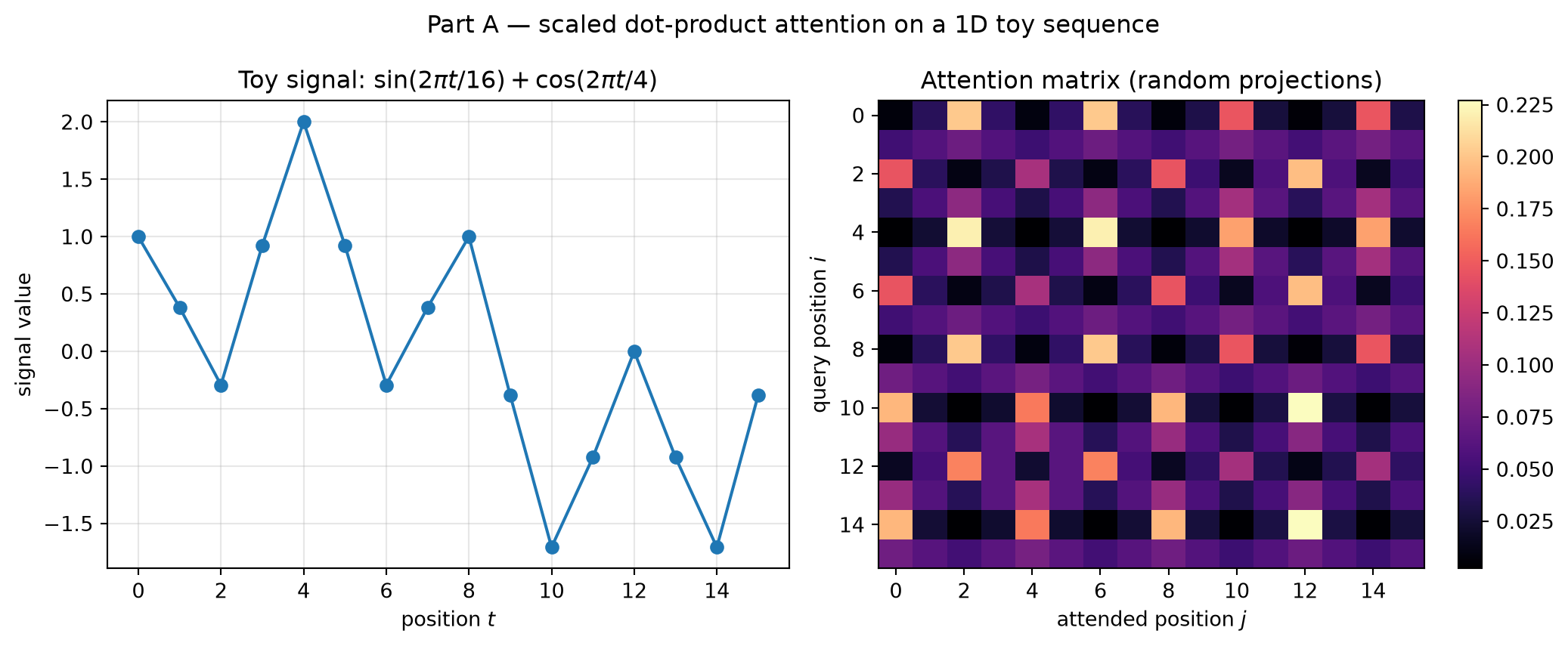
Part A: the toy-sequence attention matrix as a heatmap; verify rows sum to 1 (printed check).
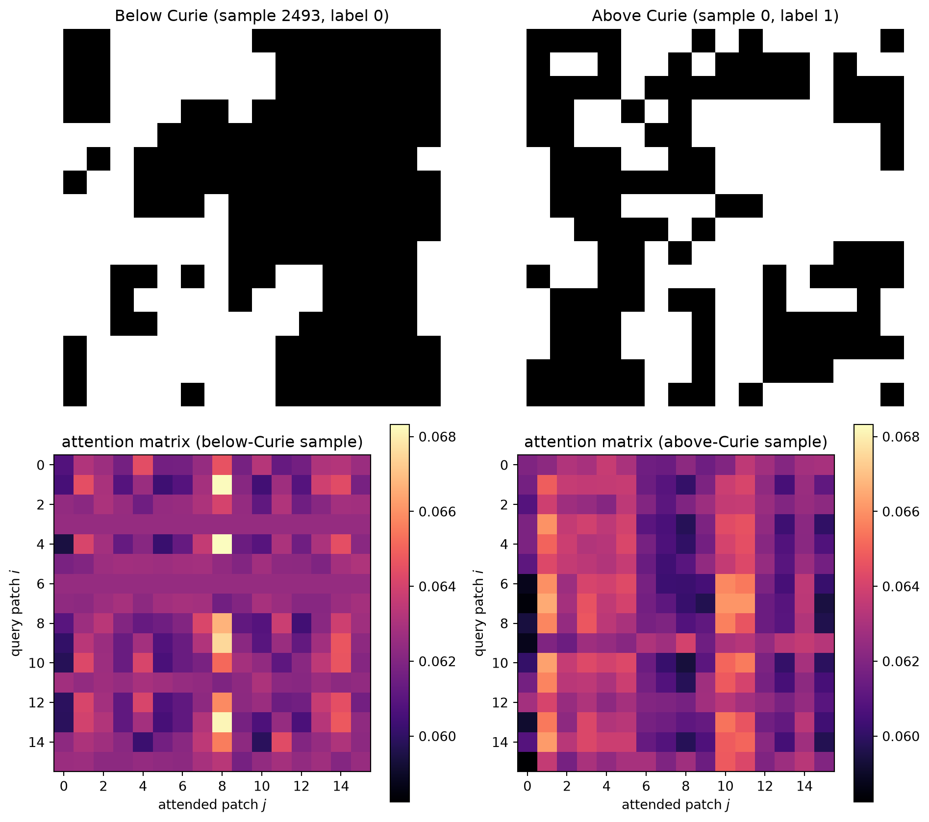
Part B: two attention-matrix heatmaps side-by-side — one above-Curie sample (random microstructure), one below-Curie sample (clustered domains).
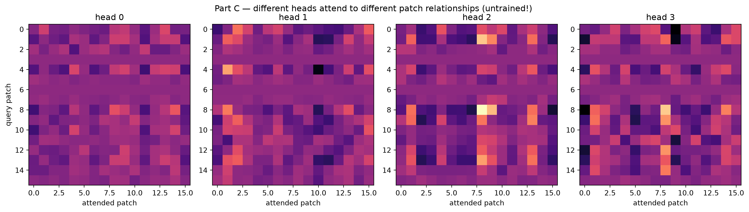
Part C: a 4-panel grid of attention maps from the four heads on the same Ising sample.
Part D: the printed composition-collision check (two prototypes, one Magpie vector) and the printed sum/mean pooling cell-doubling table — the two numbers Thursday’s GNN must respect.
Part E: your written reflection paragraph (4-6 sentences).
# Standard imports for the whole homework.import numpy as npimport torchimport torch.nn as nnimport torch.nn.functional as Fimport matplotlib.pyplot as pltfrom ai4mat.datasets import IsingDataset, CrystalGraphsDataset, MatBenchDatasetnp.random.seed(0)torch.manual_seed(0)
<torch._C.Generator at 0x7f1930f8d8b0>
Part A — Scaled dot-product attention from scratch
Self-attention takes a sequence of tokens \(\mathbf{x}_1, \dots, \mathbf{x}_T\) and produces a new sequence of tokens of the same length, where each output is a content-weighted average of the input value vectors: \[
\mathrm{Attention}(Q, K, V) = \mathrm{softmax}\!\left(\frac{QK^\top}{\sqrt{d_k}}\right) V.
\] The matrices \(Q = X W_Q\), \(K = X W_K\), \(V = X W_V\) are linear projections of the input. For each row \(i\), the attention weight on row \(j\) is proportional to the dot-product similarity of \(Q_i\) and \(K_j\), normalised by softmax.
Your task. Implement attention as a single 8-line function on a toy signal where you can read attention off the figure: a length-16 signal \(f(t) = \sin(2\pi t / 16) + \cos(2\pi t / 4)\). The slow-mode component repeats every 16 samples; the fast-mode component every 4. A randomly initialised attention layer (no training!) already shows this periodicity, because positions with similar \(K\) vectors land similar attention weights.
def scaled_dot_product_attention(Q: torch.Tensor, K: torch.Tensor, V: torch.Tensor, return_weights: bool=False):"""The whole transformer in one function. Q, K, V : tensors of shape (..., T, d). Returns: output of shape (..., T, d) and (optionally) the attention weight matrix of shape (..., T, T). """ d_k = Q.size(-1) scores = (Q @ K.transpose(-2, -1)) / np.sqrt(d_k) # (..., T, T) weights = F.softmax(scores, dim=-1) # (..., T, T) out = weights @ V # (..., T, d)if return_weights:return out, weightsreturn out
# Build the toy signal and lift each sample into a 1-D "token"T_seq =16t = np.arange(T_seq)signal = np.sin(2* np.pi * t / T_seq) + np.cos(2* np.pi * t /4)# Each token is a tiny feature vector. We use [signal_value, sin_phase, cos_phase]# so the attention layer has something non-trivial to compare on.X_np = np.stack([signal, np.sin(2* np.pi * t / T_seq), np.cos(2* np.pi * t /4)], axis=1).astype(np.float32)X = torch.tensor(X_np) # (16, 3)print(f"Part A — input X shape: {X.shape}")# Random projections: Q, K, V each in R^{d_k}. We pick d_k=3 so we can read off# what is happening. In a real transformer, d_k might be 64 per head.d_k =3W_Q = torch.randn(3, d_k)W_K = torch.randn(3, d_k)W_V = torch.randn(3, d_k)Q = X @ W_QK = X @ W_KV = X @ W_Vout, weights = scaled_dot_product_attention(Q, K, V, return_weights=True)print(f" output shape: {out.shape} (same length, projected dim)")print(f" weights shape: {weights.shape} (T x T attention matrix)")# Diagnostic: each row of the attention matrix should sum to 1 (softmax).row_sums = weights.sum(dim=-1)print(f" row sums (should all be ~1): min = {row_sums.min():.6f}, max = {row_sums.max():.6f}")
Part A — input X shape: torch.Size([16, 3])
  output shape: torch.Size([16, 3])    (same length, projected dim)
  weights shape: torch.Size([16, 16])  (T x T attention matrix)
  row sums (should all be ~1): min = 1.000000, max = 1.000000
fig, axes = plt.subplots(1, 2, figsize=(11, 4.5))axes[0].plot(t, signal, "o-")axes[0].set_xlabel("position $t$")axes[0].set_ylabel("signal value")axes[0].set_title(r"Toy signal: $\sin(2\pi t/16)+\cos(2\pi t/4)$")axes[0].grid(alpha=0.3)im = axes[1].imshow(weights.numpy(), cmap="magma", aspect="auto")axes[1].set_xlabel("attended position $j$")axes[1].set_ylabel("query position $i$")axes[1].set_title("Attention matrix (random projections)")plt.colorbar(im, ax=axes[1])fig.suptitle("Part A — scaled dot-product attention on a 1D toy sequence")plt.tight_layout()plt.show()
Part A deliverable: the attention-matrix heatmap and the printed row-sum check.
What to notice:
Even with random projections, the heatmap is not uniform. Some positions land high attention from many queries; others land none.
With trained projections (Thursday), the structure becomes meaningful: position \(i\) learns which other positions are informative for its representation.
Part B — Patchify Ising-light, attend over the 16 patches
A 16×16 Ising image becomes a sequence of 16 tokens by carving it into a 4×4 grid of 4×4-pixel patches. Each patch (16 pixels) is linearly projected to \(d_\text{model}\). The output is a sequence of shape \((16, d_\text{model})\) — exactly the same shape attention expects in Part A. From the model’s point of view, image and toy signal are the same kind of object.
Below-Curie samples have clustered black/white domains; above-Curie samples are speckled. Even with random attention projections, you should see the attention structure differ between the two classes — patches from one domain attend strongly to patches from the same domain.
ising = IsingDataset(size="light")print(f"Part B — IsingDataset(size='light'): {len(ising)} samples, X shape {ising.X.shape}, y shape {ising.y.shape}")# Pick one above-Curie sample (label 1) and one below-Curie sample (label 0).labels_np = ising.y.numpy()i_below =int(np.where(labels_np ==0)[0][0])i_above =int(np.where(labels_np ==1)[0][0])img_below = ising.X[i_below, 0].numpy() # (16, 16)img_above = ising.X[i_above, 0].numpy()
Part B — IsingDataset(size='light'): 5000 samples, X shape torch.Size([5000, 1, 16, 16]), y shape torch.Size([5000])
Part B deliverable: the four-panel figure (two images, two attention matrices) above.
Even with random projections, the two attention matrices look different because the underlying patch embeddings differ: clustered domains produce groups of similar patches that attend to each other, while a random microstructure produces a more uniform attention pattern. After training (Thursday Block 3) the contrast will be dramatic.
Part C — Multi-head attention from scratch
A single attention head sees only one similarity geometry; it cannot simultaneously notice “patches from the same domain” and “patches at the same row”. Multi-head attention runs \(H\) independent attention operations on different projected subspaces, then concatenates and linearly mixes the outputs: \[
\mathrm{MHA}(X) = \big[\mathrm{head}_1, \ldots, \mathrm{head}_H\big] W_O,
\qquad
\mathrm{head}_h = \mathrm{Attention}(X W_Q^h, X W_K^h, X W_V^h).
\] Each head has its own \(d_\text{model}/H\)-dimensional projection. Output shape stays \((T, d_\text{model})\).
Your task. Implement multi-head attention with \(H = 4\) heads. Apply it to the same below-Curie Ising sample as Part B. Plot the four attention matrices side-by-side. Different heads should produce visibly different attention patterns.
class MultiHeadSelfAttention(nn.Module):"""A from-scratch multi-head self-attention layer (no PyTorch shortcuts). The whole point of this exercise is that there are no surprises: the only operations are linear projections, einsum reshapes, and softmax. Read every line. """def__init__(self, d_model: int, n_heads: int):super().__init__()assert d_model % n_heads ==0, "d_model must divide evenly into n_heads"self.d_model = d_modelself.n_heads = n_headsself.d_head = d_model // n_headsself.W_Q = nn.Linear(d_model, d_model, bias=False)self.W_K = nn.Linear(d_model, d_model, bias=False)self.W_V = nn.Linear(d_model, d_model, bias=False)self.W_O = nn.Linear(d_model, d_model, bias=False)def forward(self, X, return_weights: bool=False):# X: (B, T, d_model). Always operate with a leading batch dim.if X.dim() ==2: X = X.unsqueeze(0) B, T, D = X.shape H, dh =self.n_heads, self.d_head Q =self.W_Q(X).view(B, T, H, dh).transpose(1, 2) # (B, H, T, dh) K =self.W_K(X).view(B, T, H, dh).transpose(1, 2) V =self.W_V(X).view(B, T, H, dh).transpose(1, 2) scores = (Q @ K.transpose(-2, -1)) / np.sqrt(dh) # (B, H, T, T) weights = F.softmax(scores, dim=-1) # (B, H, T, T) per_head = weights @ V # (B, H, T, dh) per_head = per_head.transpose(1, 2).contiguous().view(B, T, D) out =self.W_O(per_head) # (B, T, D)if return_weights:return out, weightsreturn out
torch.manual_seed(0)mha = MultiHeadSelfAttention(d_model=32, n_heads=4)# Re-embed the below-Curie image with a learnable Linear (still untrained).patch_embed = nn.Linear(d_in, d_model, bias=False)torch.manual_seed(0)patch_embed.weight.data.mul_(0.5) # smaller init for nicer-looking attentionwith torch.no_grad(): tokens_below = patch_embed(patchify(torch.tensor(img_below, dtype=torch.float32))) tokens_below = tokens_below.unsqueeze(0) # add batch dim out_mha, weights_mha = mha(tokens_below, return_weights=True)print(f"Part C — multi-head output shape: {out_mha.shape} (B, T, d_model)")print(f" weights shape: {weights_mha.shape} (B, H, T, T)")
# Visualise the four heads' attention on the same sample.fig, axes = plt.subplots(1, 4, figsize=(15, 4))W = weights_mha[0].detach().numpy() # (4, 16, 16)vmin, vmax = W.min(), W.max()for h inrange(4): im = axes[h].imshow(W[h], cmap="magma", vmin=vmin, vmax=vmax) axes[h].set_title(f"head {h}") axes[h].set_xlabel("attended patch")axes[0].set_ylabel("query patch")fig.suptitle("Part C — different heads attend to different patch relationships (untrained!)")plt.tight_layout()plt.show()
Part C deliverable: the four-panel attention-head grid above.
Different heads already differ visibly because each one’s \(W_Q^h\), \(W_K^h\), \(W_V^h\) are independently random. After training, each head learns to specialise. ML interpretability research (Vaswani 2017 Figs. 3-5; Vig 2019 BertViz) lives off looking at these.
Part D — MG-U9 prep: a crystal is a graph, not a vector
Parts A-C lived entirely in MFML’s world: tokens, attention, images. Thursday’s second thread is MG Unit 9 — Neural Networks for Materials Properties, where the input is no longer an image but an atomic system. The single idea MG-U9 starts from:
A crystal is not a vector and not an image. It is a graph of atoms under periodic boundary conditions, with four symmetries the network must respect: translation, rotation, permutation, and periodicity (MG-U9 §08).
This part is light scaffolding — no training, no GNN yet. You just load the crystal-graph dataset Thursday uses, and reproduce two load-bearing MG-U9 facts numerically so the main-notebook GNN (Block 5/6) has a concrete target to beat:
The MLP-on-Magpie failure (MG-U9 §07). A composition-only feature vector cannot distinguish two polymorphs with the same chemistry — the diamond-vs-graphite wall.
Sum (extensive) vs mean (intensive) pooling (MG-U9 §11). Permutation-invariant aggregation over atoms is the correct materials symmetry, but choosing sum vs mean is a physics decision: pick the wrong one and the model silently breaks across cell sizes.
# A crystal graph: per-atom atomic numbers Z, plus distance-labelled# edges. No grid, no fixed length — every crystal has a different atom# count. This is the data type every model in MG-U9 consumes.cg = CrystalGraphsDataset(n_total=200, seed=0)print(f"Part D — CrystalGraphsDataset: {len(cg)} crystals, "f"prototypes {cg.prototype_names}")print(f" formation-energy range = [{cg.y.min():.3f}, {cg.y.max():.3f}] eV/atom")print(f" example crystal 0: {len(cg.species[0])} atoms, "f"Z = {cg.species[0].tolist()}, "f"{cg.edge_index[0].shape[1]} directed edges")print(f" -> variable atom count per crystal: this is a *graph*, not a "f"fixed-length vector.")
Part D — CrystalGraphsDataset: 200 crystals, prototypes ['rocksalt', 'zincblende', 'wurtzite', 'fluorite', 'perovskite']
  formation-energy range = [-3.289, -1.460] eV/atom
  example crystal 0: 8 atoms, Z = [38, 38, 38, 38, 33, 33, 33, 33], 24 directed edges
  -> variable atom count per crystal: this is a *graph*, not a fixed-length vector.
Part D.1 — Composition is not enough (the MG-U9 §07 wall)
A “Magpie-style” baseline turns a crystal into a fixed vector of pooled elemental statistics (mean/std/min/max of electronegativity and covalent radius, plus atom count). It is blind to structure by construction. The dataset contains pairs of crystals with identical composition but different prototypes (e.g. rocksalt vs zincblende SnSe) — the toy analogue of diamond vs graphite. Their Magpie vectors are bitwise identical, yet their formation energies differ. No model fed only that vector can ever tell them apart.
from ai4mat.datasets.crystal_graphs import _ELECTRONEGATIVITY, _RADIUSdef magpie_vector(species) -> np.ndarray:"""Pooled elemental statistics — the Magpie recipe in miniature.""" chi = np.array([_ELECTRONEGATIVITY[int(z)] for z in species.tolist()]) rad = np.array([_RADIUS[int(z)] for z in species.tolist()])return np.array([chi.mean(), chi.std(), chi.min(), chi.max(), rad.mean(), rad.std(), rad.min(), rad.max(),float(len(species))], dtype=np.float32)# Search for two crystals with the same atom multiset but different# prototypes (we do not hard-code indices — find them honestly).by_composition = {}collision =Nonefor i inrange(len(cg)): key =tuple(sorted(cg.species[i].tolist())) proto_i =int(cg.prototype[i])if key in by_composition and by_composition[key][1] != proto_i: collision = (by_composition[key][0], i)break by_composition.setdefault(key, (i, proto_i))assert collision isnotNone, "expected a same-composition prototype collision"a, b = collisionv_a, v_b = magpie_vector(cg.species[a]), magpie_vector(cg.species[b])print(f"Part D.1 — composition collision: crystals {a} and {b}")print(f" crystal {a}: prototype '{cg.prototype_names[int(cg.prototype[a])]}', "f"Ef = {cg.y[a]:.4f} eV/atom")print(f" crystal {b}: prototype '{cg.prototype_names[int(cg.prototype[b])]}', "f"Ef = {cg.y[b]:.4f} eV/atom")print(f" same atom multiset? {sorted(cg.species[a].tolist()) ==sorted(cg.species[b].tolist())}")print(f" Magpie vectors identical? {np.allclose(v_a, v_b)} "f"<- the model's *entire* input is the same")print(f" but |Ef(a) - Ef(b)| = {abs(cg.y[a] - cg.y[b]):.4f} eV/atom "f"<- the targets are NOT")print(f" => a composition-only model is blind to the prototype "f"(MG-U9 §07,\n the diamond-vs-graphite wall). Only a "f"structure-aware model can win.")
Part D.1 — composition collision: crystals 8 and 44
  crystal 8: prototype 'rocksalt', Ef = -2.5198 eV/atom
  crystal 44: prototype 'zincblende', Ef = -1.9993 eV/atom
  same atom multiset?         True
  Magpie vectors identical?   True   <- the model's *entire* input is the same
  but |Ef(a) - Ef(b)|         = 0.5204 eV/atom   <- the targets are NOT
  => a composition-only model is blind to the prototype (MG-U9 §07,
     the diamond-vs-graphite wall). Only a structure-aware model can win.
Part D.2 — Permutation invariance, and sum vs mean pooling
A GNN turns each atom into a feature vector, then aggregates over atoms to get one crystal-level number. That aggregation must be symmetric — relabelling the atoms cannot change the prediction (MG-U9 §08, symmetry 3; §11). Sum and mean are both permutation invariant, but they behave differently when the cell is doubled:
Mean is intensive: invariant under cell doubling. Correct for per-atom formation energy, band gap, density of states.
Sum is extensive: doubles under cell doubling. Correct for total energy, total magnetisation.
We do not have a trained network yet, so we test the pooling rule directly on a stand-in per-atom feature (here: each atom’s electronegativity). Doubling the cell must leave the mean unchanged and roughly double the sum. This is the exact invariant Thursday’s GNN readout has to get right (main notebook Block 6).
def per_atom_feature(species) -> np.ndarray:"""Stand-in for a learned per-atom embedding: one scalar per atom."""return np.array([_ELECTRONEGATIVITY[int(z)] for z in species.tolist()])sp = cg.species[a]feat = per_atom_feature(sp)feat_2x = np.concatenate([feat, feat]) # the 2x supercell: atoms duplicatedsum_cell, sum_2x = feat.sum(), feat_2x.sum()mean_cell, mean_2x = feat.mean(), feat_2x.mean()# Permutation check: shuffle the atom order, both poolings must not move.rng = np.random.default_rng(0)feat_perm = feat[rng.permutation(len(feat))]print(f"Part D.2 — pooling a per-atom feature over crystal {a} "f"({len(sp)} atoms):")print(f" {'pooling':<14}{'unit cell':>12}{'2x supercell':>14}{'drift':>10}")print(f" {'mean (intensive)':<14}{mean_cell:>12.4f}{mean_2x:>14.4f} "f"{abs(mean_2x - mean_cell):>10.2e}")print(f" {'sum (extensive)':<14}{sum_cell:>12.4f}{sum_2x:>14.4f} "f"{abs(sum_2x - sum_cell):>10.2e}")print(f" permutation check (must be ~0): "f"|mean - mean(shuffled)| = {abs(feat.mean() - feat_perm.mean()):.2e}, "f"|sum - sum(shuffled)| = {abs(feat.sum() - feat_perm.sum()):.2e}")print(f" => both poolings are permutation invariant; only *mean* is "f"invariant\n under cell doubling. For per-atom formation "f"energy, mean is correct\n (MG-U9 §11). Picking sum here "f"silently breaks cell-size transfer.")
Part D.2 — pooling a per-atom feature over crystal 8 (8 atoms):
  pooling           unit cell   2x supercell      drift
  mean (intensive)       2.2550         2.2550   0.00e+00
  sum  (extensive)      18.0400        36.0800   1.80e+01
  permutation check (must be ~0): |mean - mean(shuffled)| = 0.00e+00, |sum - sum(shuffled)| = 0.00e+00
  => both poolings are permutation invariant; only *mean* is invariant
     under cell doubling. For per-atom formation energy, mean is correct
     (MG-U9 §11). Picking sum here silently breaks cell-size transfer.
Part D deliverable: the two printed blocks above —
the composition-collision check (same Magpie vector, different formation energy), and
the sum-vs-mean cell-doubling table (mean invariant, sum doubles, both permutation invariant).
These are the two numbers Thursday’s from-scratch crystal-graph GNN (main notebook Block 5/6) must respect: it must beat the composition-only baseline (because it sees structure), and it must use mean pooling so the per-atom energy stays invariant under cell doubling. You are not asked to build the GNN here — only to understand why a plain vector model cannot, and what symmetry the pooling encodes.
Part D.3 — The same ceiling on a real benchmark (one cell)
D.1 showed the composition-collision on the toy dataset. To see it is not a synthetic artefact, here is one light real-data baseline: matbench_perovskites (~19k DFT perovskites from Materials Project). mb.X is a fixed 118-dim element-fraction vector — composition only, no structure — and mb.y is the DFT formation energy. We fit a trivial Ridge model on a seeded 3000-row slice. This is the composition-only number to put next to Thursday’s structure-aware crystal-graph GNN (main notebook Block 5b): the GNN sees the graph; this baseline only sees the chemistry, so it cannot resolve two perovskites that differ only in structure. Same wall as D.1, on real DFT data. (First run downloads ~a few MB and caches under data/.)
from sklearn.linear_model import Ridgefrom sklearn.metrics import mean_absolute_errormb = MatBenchDataset(task="matbench_perovskites", root="data/matbench", download=True)_rng_mb = np.random.default_rng(0)_k_mb =3000_sel_mb = _rng_mb.permutation(len(mb.X))[:_k_mb]Xmb = mb.X.numpy()[_sel_mb]ymb = mb.y.numpy()[_sel_mb]_sp =int(0.8* _k_mb)mb_baseline = Ridge(alpha=1.0).fit(Xmb[:_sp], ymb[:_sp])mae_mb =float(mean_absolute_error(ymb[_sp:], mb_baseline.predict(Xmb[_sp:])))print(f"Part D.3 — matbench_perovskites, composition-only Ridge baseline:")print(f" full dataset {tuple(mb.X.shape)}, seeded {_k_mb}-row slice, "f"feature dim {Xmb.shape[1]} (element fractions, NO structure)")print(f" test MAE = {mae_mb:.4f} eV/atom "f"(predict-the-mean ref {ymb[_sp:].std():.4f})")print(f" => this is the composition-only number Thursday's "f"crystal-graph GNN\n (main notebook Block 5b) must beat. It "f"learns the chemistry trend but\n is structurally blind: two "f"perovskites with the same composition and\n different "f"structure get the same input. The graph point in Part D, on\n"f" real data.")
Part D.3 — matbench_perovskites, composition-only Ridge baseline:
  full dataset (18928, 118), seeded 3000-row slice, feature dim 118 (element fractions, NO structure)
  test MAE = 0.4636 eV/atom   (predict-the-mean ref 0.7386)
  => this is the composition-only number Thursday's crystal-graph GNN
     (main notebook Block 5b) must beat. It learns the chemistry trend but
     is structurally blind: two perovskites with the same composition and
     different structure get the same input. The graph point in Part D, on
     real data.
Part E — Reflection: attention vs convolution
A convolutional layer has locality and translation equivariance baked in: a 3×3 kernel always looks at a 3×3 neighbourhood, and the same kernel is applied at every position. Attention has neither. Position-\(i\)’s representation is a content-weighted average of all positions, regardless of distance, and there is no built-in notion of “which two positions are neighbours” — the model learns that from data, with help from positional encoding.
Your task (~10 min, write 4-6 sentences):
Pick one of the following pairs and answer two questions:
Crystal-structure property prediction (graph of atoms, Part D) vs sequence prediction in linguistics. (Hint: which of the four MG-U9 symmetries does each architecture get for free?)
Microscopy denoising (lots of pixels, lots of training data) vs property prediction (few hundred materials).
Questions:
Which inductive bias — attention’s learn-everything-from-data or convolution’s built-in locality — is better suited to the problem, and why?
What is the smallest experiment you would run to test your answer?
Bring the paragraph to Thursday; we will pick two volunteers to read theirs aloud at the start of Block 1.
Hand in: your written paragraph (Markdown cell below).