This week braids the three lectures that materials students actually sit on 23.06, around one spine: a learned representation is only as good as what it lets you do downstream — generate, diagnose, automate.
MFML Unit 11: Generative models — VAE, β-VAE, conditional VAE, DDPM as historical anchor, flow matching as the 2026 default [@lipman_2023_flow_matching], consistency models for one-step sampling [@song_2023_consistency]. (Blocks 1–4, 6; the spine.)
MG Unit 10 (Representation Learning & Feature Discovery, the true calendar-W11 MG lecture): embedding diagnostics — linear probe vs random-init baseline vs engineered (Magpie-style) features, nearest-neighbour retrieval, and the deck’s signature “pretty t-SNE / dead downstream” anti-pattern. The W11 deck explicitly defers generative latent arithmetic to MG U12, so Block 5 is now diagnostics, not property-targeted generation. (Block 5.)
ML-PC Unit 10 (Automation in microscopy & characterization, the true calendar-W11 ML-PC lecture): an autonomous acquire → model → decide → acquire loop — active-learning / self-driving-lab style, with the deck’s conformal automate/escalate decision rule. (Block 5b.)
Red thread:Week 9 read the latent space; today we use it three ways. MFML supplies the VAE/diffusion machinery to generate candidates. MG supplies the discipline to diagnose whether a learned embedding is actually doing work (probe before you trust). ML-PC closes the loop: an embedding good enough to retrieve in is good enough to steer an autonomous experiment — the self-driving-lab loop that decides what to measure next.
Pre-flight check. This notebook assumes you have run notebooks/week11_homework.py. Block 1 picks up directly from your Part B β-VAE curves and your Part C interpolation grid.
Agenda (90 min)
Block
Min
Topic
1
~5
Recap from homework — VAE, ELBO, β trade-off
2
~12
Conditional VAE on Cahn–Hilliard — generation under target free energy
3
~12
Latent-space gradient descent — inverse design as differentiable optimization
The VAE compresses CH microstructure into 8 latent dimensions from which the decoder regenerates plausible images.
β controls the trade-off: small β → busy, expressive latent; large β → near-prior latent at the cost of reconstruction quality.
The latent space is smooth: walking from \(z_{\text{low E}}\) to \(z_{\text{high E}}\) produces a continuous sequence of plausible microstructures, not a sequence of nearest-neighbour copies.
Today we use that smoothness for inverse design: given a target free energy, can we find a latent that decodes to a microstructure with that energy? Two methods:
Conditional VAE (Block 2): bake the target into the model.
Latent-space gradient descent (Block 3): freeze the model, solve for \(z\) at inference time.
# Quick warm-up: train an unconditional VAE that we will reuse in Blocks# 3 and 6 (for the latent-GD baseline and the failure-mode demos).print("Pretraining unconditional VAE for downstream blocks...")torch.manual_seed(0)vae = TinyVAE(latent_dim=8).to(DEVICE)opt = torch.optim.Adam(vae.parameters(), lr=1e-3)loader = DataLoader(TensorDataset(X_tr), batch_size=64, shuffle=True)for ep inrange(4): vae.train() losses = []for (xb,) in loader: x_hat, mu, log_var, _ = vae(xb) loss, _, _ = vae_loss(xb, x_hat, mu, log_var, beta=1.0) opt.zero_grad(); loss.backward(); opt.step() losses.append(loss.item())print(f" epoch {ep} total ELBO loss = {np.mean(losses):.4f}")
Pretraining unconditional VAE for downstream blocks...
  epoch 0  total ELBO loss = 582.8805
  epoch 1  total ELBO loss = 362.3943
  epoch 2  total ELBO loss = 179.8163
  epoch 3  total ELBO loss = 106.5870
Block 2 — Conditional VAE on Cahn-Hilliard
A conditional VAE is the cleanest form of property-targeted generation: append the target \(y\) to both the encoder input and the decoder input. Concretely:
encoder: \(q_\phi(z \mid x, y)\)
decoder: \(p_\theta(x \mid z, y)\)
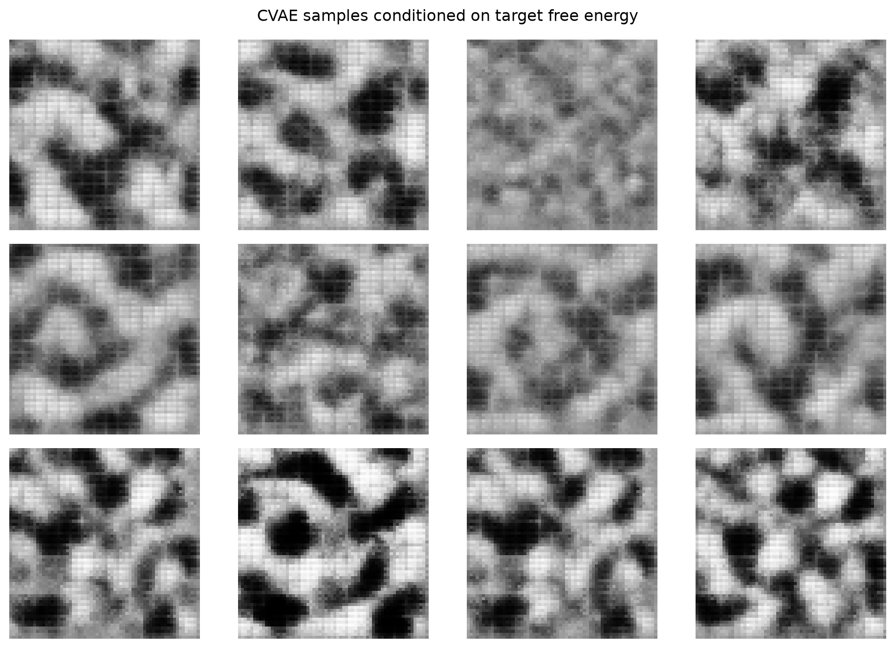
At inference, sample \(z \sim \mathcal{N}(0, I)\), pick any \(y^*\), decode \(\hat x = \text{dec}(z, y^*)\). This is the simplest “give me a sample with energy = X” pipeline.
(see ML-PC §“VAE-based inverse design”, §“Conditional generation under target property”; MFML §“Conditional VAE”)
class TinyCVAE(nn.Module):"""Conditional VAE. The condition y is broadcast as a constant feature map and concatenated with the input image (encoder side); on the decoder side it is concatenated with z."""def__init__(self, latent_dim=8):super().__init__()self.latent_dim = latent_dimself.enc_conv = nn.Sequential( nn.Conv2d(2, 16, 3, stride=2, padding=1), nn.ReLU(), # 2 channels: image + y-broadcast nn.Conv2d(16, 32, 3, stride=2, padding=1), nn.ReLU(), )self.enc_lin = nn.Linear(32*16*16, 2* latent_dim)self.dec_lin = nn.Linear(latent_dim +1, 32*16*16) # +1 for yself.dec_conv = nn.Sequential( nn.ConvTranspose2d(32, 16, 3, stride=2, padding=1, output_padding=1), nn.ReLU(), nn.ConvTranspose2d(16, 1, 3, stride=2, padding=1, output_padding=1), nn.Sigmoid(), )def encode(self, x, y):# broadcast y as a 64x64 feature plane y_plane = y.view(-1, 1, 1, 1).expand(-1, 1, x.shape[2], x.shape[3]) h =self.enc_conv(torch.cat([x, y_plane], dim=1)).flatten(1)returnself.enc_lin(h).chunk(2, dim=-1)def decode(self, z, y): zy = torch.cat([z, y.view(-1, 1)], dim=1)returnself.dec_conv(self.dec_lin(zy).view(-1, 32, 16, 16))def forward(self, x, y): mu, log_var =self.encode(x, y) z = mu + torch.exp(0.5* log_var) * torch.randn_like(mu)returnself.decode(z, y), mu, log_var, z
Training CVAE on (image, energy) pairs...
  epoch 0  total ELBO loss = 594.9465
  epoch 1  total ELBO loss = 400.2399
  epoch 2  total ELBO loss = 189.2807
  epoch 3  total ELBO loss = 112.0297
Target energies (de-normalised): low = 467, median = 630, high = 1094
What you should see. Across the three rows, the microstructures differ visibly: at low target energy, the patterns are well-separated phase domains; at high target energy, the patterns are noisier with more interface area (CH thermodynamics: higher energy = more interface). Within a row, the four samples are different but similar — the VAE generates diverse candidates that all share the target property.
This is the cleanest form of inverse design: one model, two minutes of training, and a control knob that produces property-targeted samples on demand.
Block 3 — Latent-space gradient descent (inverse design as optimization)
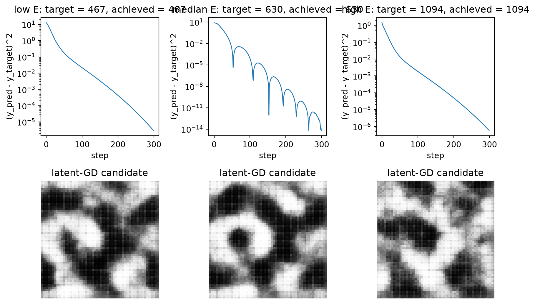
An alternative recipe: don’t retrain the VAE — instead, use the frozen unconditional VAE plus a frozen property regressor, and solve for the latent that gives the target property by gradient descent.
The chain z → decode → regressor → property is fully differentiable, so this is a 5-line training loop. The advantage: works on any pretrained generator + regressor, no joint retraining required. The disadvantage: each target \(y^*\) requires its own optimisation (the CVAE amortises this).
(see ML-PC §“Latent optimization for inverse design”; MFML §“Differentiable generation”)
# Train a small CNN regressor on (image, energy) for use in Block 3.class EnergyRegressor(nn.Module):def__init__(self):super().__init__()self.net = nn.Sequential( nn.Conv2d(1, 16, 3, stride=2, padding=1), nn.ReLU(), nn.Conv2d(16, 32, 3, stride=2, padding=1), nn.ReLU(), nn.AdaptiveAvgPool2d(4), nn.Flatten(), nn.Linear(32*16, 64), nn.ReLU(), nn.Linear(64, 1), )def forward(self, x):returnself.net(x).squeeze(-1)print("Training energy regressor on CH images...")torch.manual_seed(0)reg = EnergyRegressor().to(DEVICE)opt = torch.optim.Adam(reg.parameters(), lr=1e-3)loader_reg = DataLoader(TensorDataset(X_tr, y_tr_n), batch_size=64, shuffle=True)for ep inrange(4): reg.train() losses = []for xb, yb in loader_reg: opt.zero_grad() loss = F.mse_loss(reg(xb), yb) loss.backward(); opt.step() losses.append(loss.item())print(f" epoch {ep} train MSE = {np.mean(losses):.4f}")with torch.no_grad(): test_mae = (reg(X_te) - y_te_n).abs().mean().item() * y_stdprint(f" test MAE (de-normalised): {test_mae:.1f} energy units")
Training energy regressor on CH images...
  epoch 0  train MSE = 0.9437
  epoch 1  train MSE = 0.4889
  epoch 2  train MSE = 0.1148
  epoch 3  train MSE = 0.0870
  test MAE (de-normalised): 26.7 energy units
def latent_gd(target_y_n, n_steps=300, lr=0.05):"""Gradient-descend in z for a target normalised energy. Frozen unconditional VAE decoder + frozen regressor; only z requires grad. """ z = torch.randn(1, vae.latent_dim, device=DEVICE, requires_grad=True) opt_z = torch.optim.Adam([z], lr=lr) target = torch.tensor([target_y_n], device=DEVICE) losses = []for _ inrange(n_steps): opt_z.zero_grad() x_hat = vae.decode(z) y_pred = reg(x_hat) loss = (y_pred - target).pow(2).mean() loss.backward(); opt_z.step() losses.append(loss.item())return z.detach(), losses# Run latent-GD for the three target energies and visualise.fig, axes = plt.subplots(2, 3, figsize=(9, 5.5))for r, (yt, lbl) inenumerate(zip(targets_n, target_labels)): z_star, loss_curve = latent_gd(yt)with torch.no_grad(): x_star = vae.decode(z_star) y_pred = reg(x_star).item() axes[0, r].plot(loss_curve, lw=1.0) axes[0, r].set_yscale("log") axes[0, r].set_title(f"{lbl}: target = {yt*y_std+y_mean:.0f}, achieved = {y_pred*y_std+y_mean:.0f}") axes[0, r].set_xlabel("step"); axes[0, r].set_ylabel("(y_pred - y_target)^2") axes[1, r].imshow(x_star[0, 0].cpu().numpy(), cmap="gray", vmin=0, vmax=1) axes[1, r].axis("off"); axes[1, r].set_title(f"latent-GD candidate")plt.tight_layout(); plt.show()
CVAE vs latent-GD — which wins? Both produce candidates with the target energy. The CVAE produces diverse candidates per call (different z, same y); latent-GD produces a deterministic candidate per random init. Latent-GD requires no retraining — useful when a new target is requested at inference time. CVAE amortises the optimisation — useful when many targets need many samples.
Real-world materials inverse design uses both: a CVAE for proposal generation, latent-GD for refinement.
Block 4 — Flow matching for inverse design
Pedagogical anchor — DDPM then flow matching. The other major generative family used to be DDPM (denoising diffusion probabilistic models): an SDE-based generator with a noisy forward process
and a learned, stochastic, 1000-step reverse process that predicts the noise \(\varepsilon_\theta(x_t, t)\). DDPM is what got the field excited in 2020; we keep the equation above as a historical anchor and move on.
In 2026 the default new image generator is flow matching[@lipman_2023_flow_matching]: an ODE-based generator with a simpler loss and fewer sampling steps. Same U-Net backbone, different training target. The recipe is:
Forward path (no learning): sample \(x_0 \sim \mathcal{N}(0, I)\) and \(x_1\) from data. Sample \(t \sim \mathrm{Uniform}(0, 1)\) and form the linear interpolant \(x_t = (1 - t) x_0 + t x_1\).
Sample: start from \(x \leftarrow x_0 \sim \mathcal{N}(0, I)\) and integrate the learned ODE \(\dot x = u_\theta(x, t)\) from \(t = 0\) to \(t = 1\) with a small number of solver steps.
DDPM and flow matching share the U-Net; flow matching replaces “predict noise on a noisy schedule” with “predict the straight-line velocity”, which trains faster and samples in 10 ODE steps instead of hundreds.
(see MFML §“Flow matching”; ML-PC §“Flow-matching microstructure inverse design”)
# Visualise the linear interpolant x_t = (1-t) x_0 + t x_1 used by flow# matching. No training; just forward path inspection.x1_demo = X_tr[0:1] # one data samplex0_demo = torch.randn_like(x1_demo) # one Gaussian samplet_show = [0.0, 0.2, 0.4, 0.6, 0.8, 1.0]fig, axes = plt.subplots(1, 6, figsize=(13, 2.5))for i, t_i inenumerate(t_show): x_t_demo = (1- t_i) * x0_demo + t_i * x1_demo axes[i].imshow(x_t_demo[0, 0].cpu().numpy(), cmap="gray") axes[i].set_title(f"t = {t_i:.1f}", fontsize=9); axes[i].axis("off")plt.suptitle("Flow-matching interpolant x_t = (1-t) x_0 + t x_1 (no training)")plt.tight_layout(); plt.show()
class TinyUNet(nn.Module):"""Minimal U-Net for the flow-matching velocity field. 64x64 in/out; sinusoidal time embedding; channel mults [16, 32, 64]. Same architecture we used for DDPM in the 2025 edition of this notebook — flow matching only changes the *loss* and *sampler*, not the backbone."""def__init__(self, time_dim=64):super().__init__()self.time_dim = time_dimself.time_mlp = nn.Sequential( nn.Linear(time_dim, 128), nn.SiLU(), nn.Linear(128, 128), )self.in_conv = nn.Conv2d(1, 16, 3, padding=1)self.down1 = nn.Sequential(nn.Conv2d(16, 32, 3, stride=2, padding=1), nn.SiLU())self.down2 = nn.Sequential(nn.Conv2d(32, 64, 3, stride=2, padding=1), nn.SiLU())self.mid = nn.Sequential( nn.Conv2d(64, 64, 3, padding=1), nn.SiLU(), nn.Conv2d(64, 64, 3, padding=1), nn.SiLU(), )self.up2 = nn.Sequential(nn.ConvTranspose2d(64, 32, 4, stride=2, padding=1), nn.SiLU())self.up1 = nn.Sequential(nn.ConvTranspose2d(32, 16, 4, stride=2, padding=1), nn.SiLU())self.out_conv = nn.Conv2d(16, 1, 3, padding=1)# Project time embedding into each scale.self.time_proj_mid = nn.Linear(128, 64)self.time_proj_up2 = nn.Linear(128, 32)self.time_proj_up1 = nn.Linear(128, 16)def time_embedding(self, t):"""t is a continuous tensor in [0, 1] here (flow matching), not an integer step index as it was in DDPM. We rescale to keep the sinusoidal frequencies in a useful range.""" half =self.time_dim //2 freqs = torch.exp(-math.log(10000) * torch.arange(half, device=t.device) / half) args = (t.float() *1000.0)[:, None] * freqs[None]return torch.cat([args.sin(), args.cos()], dim=-1)def forward(self, x, t): t_emb =self.time_mlp(self.time_embedding(t)) # (B, 128) h0 =self.in_conv(x) # (B, 16, 64, 64) h1 =self.down1(h0) # (B, 32, 32, 32) h2 =self.down2(h1) # (B, 64, 16, 16) h_mid =self.mid(h2 +self.time_proj_mid(t_emb)[:, :, None, None]) u2 =self.up2(h_mid) u2 = u2 + h1 # skip u1 =self.up1(u2 +self.time_proj_up2(t_emb)[:, :, None, None]) u1 = u1 + h0returnself.out_conv(u1 +self.time_proj_up1(t_emb)[:, :, None, None])
if HAS_GPU:print("GPU detected — training tiny flow-matching U-Net (~1-2 min on 1080Ti)") torch.manual_seed(0) unet = TinyUNet().to(DEVICE) opt = torch.optim.Adam(unet.parameters(), lr=2e-4) loader_fm = DataLoader(TensorDataset(X_tr), batch_size=32, shuffle=True) n_epochs_fm =20for ep inrange(n_epochs_fm): unet.train() losses = []for (xb,) in loader_fm:# Flow-matching loss: predict the straight-line velocity. x1 = xb x0 = torch.randn_like(x1) t = torch.rand(x1.shape[0], device=DEVICE) x_t = (1- t).view(-1, 1, 1, 1) * x0 + t.view(-1, 1, 1, 1) * x1 u_star = x1 - x0 # target velocity u_pred = unet(x_t, t) loss = F.mse_loss(u_pred, u_star) opt.zero_grad(); loss.backward(); opt.step() losses.append(loss.item())if ep %4==0or ep == n_epochs_fm -1:print(f" epoch {ep:2d} velocity-matching MSE = {np.mean(losses):.4f}")# Sample with a 10-step Heun ODE solver (predictor + corrector).@torch.no_grad()def fm_sample_heun(unet, n=6, n_steps=10):"""Heun's method for x' = u_theta(x, t), t: 0 -> 1. Each step does a predictor (Euler) and a corrector (average of velocities at both ends). 10 steps is plenty for this small model — that's the flow-matching efficiency story.""" x = torch.randn(n, 1, 64, 64, device=DEVICE) ts = torch.linspace(0.0, 1.0, n_steps +1, device=DEVICE)for k inrange(n_steps): t_k = ts[k]; t_k1 = ts[k +1] dt = t_k1 - t_k t_vec = torch.full((n,), float(t_k), device=DEVICE) u_k = unet(x, t_vec) # predictor velocity x_pred = x + dt * u_k # Euler step t_vec1 = torch.full((n,), float(t_k1), device=DEVICE) u_k1 = unet(x_pred, t_vec1) # corrector velocity x = x +0.5* dt * (u_k + u_k1) # Heun averagereturn x.clamp(0, 1) samples = fm_sample_heun(unet, n=6, n_steps=10) fig, axes = plt.subplots(1, 6, figsize=(13, 2.5))for i inrange(6): axes[i].imshow(samples[i, 0].cpu().numpy(), cmap="gray", vmin=0, vmax=1) axes[i].axis("off"); axes[i].set_title(f"FM sample {i}", fontsize=9) plt.suptitle("Samples from the trained flow-matching ODE (10 Heun steps)") plt.tight_layout(); plt.show()else:print("No GPU detected — skipping flow-matching training.")print("The interpolant visualisation above is the qualitative point.")print("On a GPU machine, the next cell would train a tiny U-Net flow-matching")print("model in ~1-2 min and sample in 10 ODE steps.") unet =None# used by Exercise 5
No GPU detected — skipping flow-matching training.
The interpolant visualisation above is the qualitative point.
On a GPU machine, the next cell would train a tiny U-Net flow-matching
model in ~1-2 min and sample in 10 ODE steps.
Take-home from Block 4. Flow matching reaches similar visual quality to a tiny DDPM with ~10x fewer sampling steps and a simpler loss (MSE on a velocity, no noise schedule, no \(\bar\alpha_t\) bookkeeping). That’s the 2026 default for new image generators.
Flow matching vs VAE — when to pick which?
Flow matching produces sharper samples with enough training — no posterior collapse, no blurry-mean-of-modes artefact.
Flow matching is slower at sampling than a VAE (10 ODE steps vs 1 decode), but much faster than DDPM (which used hundreds of steps).
VAE sampling is one decode call — fastest — but blurrier.
Conditional generation in a CVAE is one extra input (Block 2); conditional generation in flow matching uses classifier-free guidance on the velocity field — the same idea as guided diffusion, applied to the ODE.
Where DDPM lives now. As the SDE-based ancestor: the 2 lines of math at the top of this block are the only DDPM you need today. Everything downstream — score matching, classifier-free guidance, consistency distillation — generalises naturally to the flow-matching ODE.
Block 5 — Embedding diagnostics (MG W11)
We now switch from CH images to crystal embeddings — the MG home turf. But the true MG-W11 lecture is not latent-space arithmetic for property targeting (that is explicitly deferred to MG U12, “Generative Models & Inverse Design”). MG-W11 is Representation Learning & Feature Discovery, and its conceptual centre is a discipline, not a generator:
Probe before you project. A learned embedding is only useful to the extent it contains information about the property you care about — and a pretty 2-D projection does not establish that.
We exercise the deck’s diagnostic stack on a small TinyCGNN trained on toy formation energies:
Linear probe vs random-init baseline vs engineered features (MG §F slide 42): freeze the encoder, fit a linear head on a held-out prototype, and compare against (i) a random-init encoder of the same architecture and (ii) a hand-engineered composition baseline (a Magpie-style stand-in). Without the random-init row you cannot tell whether training helped or whether the architecture did the work — “the most-omitted comparison in published work”.
Nearest-neighbour retrieval (MG §F slide 43): the diagnostic the deck trusts most — full-dimension, per-query, manually inspectable.
The “pretty t-SNE / dead downstream” trap (MG §F slide 45): construct it on purpose — a PCA scatter that looks structured while a probe of a metadata artefact (prototype id / atom count) scores high and the property probe is comparatively weak.
Protocol (MG §F slide 42). Freeze each representation. Hold out one entire prototype (here perovskite) — this is the deck’s held-out-chemistry requirement: a probe evaluated on the same distribution it was fit on is a memorisation test, not a transfer test. Fit a closed-form ridge-regression linear head on the other 4 prototypes, evaluate \(R^2\) / MAE on the held-out one. Compare four rows: trained encoder, random-init encoder, Magpie-style features, and a raw-mean-atomic-number scalar (a deliberately weak floor).
def linear_probe(Z, y, train_mask, test_mask, ridge=1.0):"""Closed-form ridge linear probe. Returns (R2, MAE) on the test set. Standardise features on the train split, append a bias, solve the normal equations with an L2 penalty (no torch grad needed).""" Z = Z.float() mu = Z[train_mask].mean(0, keepdim=True) sd = Z[train_mask].std(0, keepdim=True).clamp_min(1e-6) Zs = (Z - mu) / sd Ztr = torch.cat([Zs[train_mask], torch.ones(train_mask.sum(), 1)], dim=1) Zte = torch.cat([Zs[test_mask], torch.ones(test_mask.sum(), 1)], dim=1) ytr = y[train_mask].unsqueeze(1) d = Ztr.shape[1] reg = ridge * torch.eye(d); reg[-1, -1] =0.0# don't penalise bias w = torch.linalg.solve(Ztr.T @ Ztr + reg, Ztr.T @ ytr) yhat = (Zte @ w).squeeze(1) yte = y[test_mask] ss_res = ((yte - yhat) **2).sum() ss_tot = ((yte - yte.mean()) **2).sum().clamp_min(1e-12) r2 = (1- ss_res / ss_tot).item() mae = (yte - yhat).abs().mean().item()return r2, maeheld_out_proto = cg.prototype_names.index("perovskite")test_mask = (prototype == held_out_proto)train_mask =~test_maskprint(f"Held-out prototype: 'perovskite' "f"({int(test_mask.sum())} test / {int(train_mask.sum())} train crystals)")# A deliberately weak floor: a single per-crystal scalar (mean atomic# number). Anything that cannot beat this is not a representation.floor_feat = torch.stack([cg[i]["species"].float().mean()for i inrange(len(cg))]).unsqueeze(1) # (200,1)probe_rows = [ ("trained CGNN encoder", emb_trained), ("random-init CGNN encoder", emb_random), ("Magpie-style features", feat_magpie), ("mean-Z scalar (weak floor)", floor_feat),]print(f"\n{'representation':<30}{'R2':>7}{'MAE (eV/atom)':>14}")print("-"*56)probe_results = {}for name, Z in probe_rows: r2, mae = linear_probe(Z, y_true, train_mask, test_mask) probe_results[name] = (r2, mae)print(f"{name:<30}{r2:7.3f}{mae:14.3f}")
Reading the probe table. The row that matters most is random-init CGNN encoder. If it scores close to the trained encoder, the architecture (graph message passing + mean pooling) is doing the work and the supervised training added little — exactly the “most-omitted comparison” the MG deck (slide 42) insists on. The Magpie-style row is the engineered baseline any learned embedding must beat to justify its cost (MG §G slide 47). On this toy dataset the formation energy is largely an electronegativity/radius-mismatch function of composition, so expect the cheap composition features to be a strong baseline — the deck’s “always use the foundation model is wrong” point, measured.
5.2 — Nearest-neighbour retrieval (the honest diagnostic)
Protocol (MG §F slide 43). For each query crystal, retrieve its \(k\) nearest neighbours in full embedding dimension (no 2-D projection) and ask: do the neighbours share the query’s prototype, and are their formation energies clustered near the query’s? We report precision@k for prototype and the mean absolute energy gap to the query — the per-query, manually-inspectable diagnostic the deck trusts more than any t-SNE.
def retrieval_metrics(Z, k=5):"""Mean prototype precision@k and mean |Δenergy| to query, full-dim.""" Z = F.normalize(Z.float(), dim=1) sim = Z @ Z.T sim.fill_diagonal_(-2.0) # exclude self nn_idx = sim.topk(k, dim=1).indices # (N, k) proto_hit = (prototype[nn_idx] == prototype[:, None]).float().mean().item() e_gap = (y_true[nn_idx] - y_true[:, None]).abs().mean().item()return proto_hit, e_gapprint(f"{'representation':<30}{'proto P@5':>10}{'mean |ΔE| (eV/atom)':>20}")print("-"*64)for name, Z in [("trained CGNN encoder", emb_trained), ("random-init CGNN encoder", emb_random), ("Magpie-style features", feat_magpie)]: p_at_k, e_gap = retrieval_metrics(Z, k=5)print(f"{name:<30}{p_at_k:10.3f}{e_gap:20.3f}")# A worked example: 1 query, its 5 nearest neighbours in the trained space.Zn = F.normalize(emb_trained, dim=1)q =0sims = Zn @ Zn[q]; sims[q] =-2.0nn5 = sims.topk(5).indicesprint(f"\nQuery crystal {q}: prototype="f"{cg.prototype_names[int(prototype[q])]}, E={y_true[q]:+.2f} eV/atom")for j in nn5.tolist():print(f" neighbour {j:3d}: "f"prototype={cg.prototype_names[int(prototype[j])]:<10} "f"E={y_true[j]:+.2f} (ΔE={abs(y_true[j]-y_true[q]):.2f})")
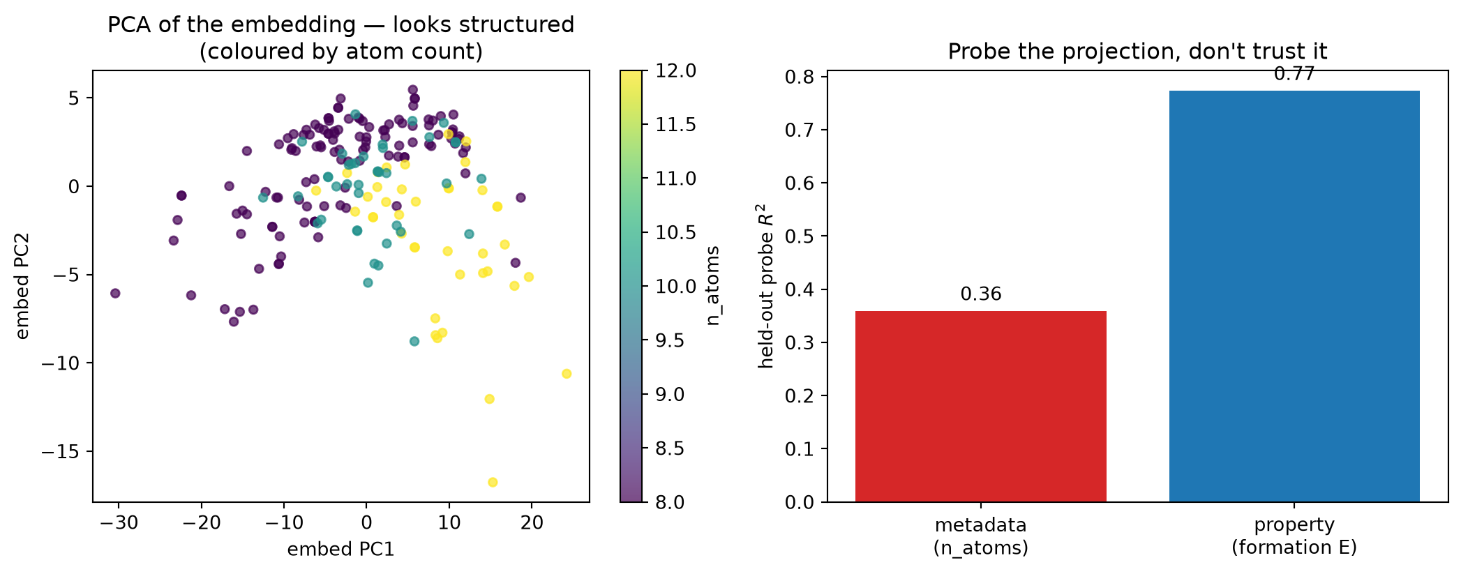
The anti-pattern (MG §F slide 45). A 2-D projection can look beautifully clustered while the embedding is useless for the property — because the projection latches onto a high-variance metadata artefact. The deck’s canonical concrete example: “the embedding had learned to count atoms — the cluster picture was by number of atoms in the cell, and the property probe was at chance.” We reproduce exactly that: the artefact is atom count per cell (n_atoms), a real but physically-irrelevant-to-stability quantity.
We PCA-scatter the trained embedding (it looks structured), then put two probes on the same random split side by side — a probe of n_atoms (the metadata artefact) vs a probe of formation energy (the property we actually want). The lesson lands when the artefact probe scores high while the property probe is comparatively weak: the projection organised the embedding by the artefact, not the property.
def pca_2d(X): X = X.float() mu = X.mean(0, keepdim=True) Xc = X - mu cov = Xc.T @ Xc / (Xc.shape[0] -1) eigvals, eigvecs = torch.linalg.eigh(cov) order = torch.argsort(eigvals, descending=True) V = eigvecs[:, order][:, :2]return Xc @ VZ2 = pca_2d(emb_trained) # (200, 2)# The metadata artefact: number of atoms in the cell — real, but# physically irrelevant to formation energy. Probe it vs the property on# the SAME random 75/25 split (both targets are in-distribution here; the# point is "same embedding, same split, artefact wins").n_atoms = torch.tensor([float(cg[i]["species"].numel())for i inrange(len(cg))])g_split = torch.Generator().manual_seed(0)perm_e = torch.randperm(len(cg), generator=g_split)n_tr_e =int(0.75*len(cg))rand_train = torch.zeros(len(cg), dtype=torch.bool)rand_train[perm_e[:n_tr_e]] =Truerand_test =~rand_trainr2_artefact, _ = linear_probe(emb_trained, n_atoms, rand_train, rand_test)r2_property, _ = linear_probe(emb_trained, y_true, rand_train, rand_test)print(f"trained-embedding probe (random split): "f"n_atoms artefact R2 = {r2_artefact:.3f} "f"formation-energy R2 = {r2_property:.3f}")fig, (a1, a2) = plt.subplots(1, 2, figsize=(11, 4.4))sc = a1.scatter(Z2[:, 0], Z2[:, 1], s=20, alpha=0.7, c=n_atoms.numpy(), cmap="viridis")a1.set_xlabel("embed PC1"); a1.set_ylabel("embed PC2")a1.set_title("PCA of the embedding — looks structured\n(coloured by atom count)")fig.colorbar(sc, ax=a1, label="n_atoms")a2.bar(["metadata\n(n_atoms)", "property\n(formation E)"], [r2_artefact, r2_property], color=["C3", "C0"])a2.axhline(0.0, c="grey", lw=0.8)a2.set_ylabel("held-out probe $R^2$")a2.set_title("Probe the projection, don't trust it")for i, v inenumerate([r2_artefact, r2_property]): a2.text(i, v +0.02* (1if v >=0else-1), f"{v:.2f}", ha="center", fontsize=10)plt.tight_layout(); plt.show()
Reading the trap. The left scatter looks like the embedding “knows something” — and the colour reveals what: the structure tracks atom count, not stability. The right panel is the honest verdict: the metadata-artefact probe (n_atoms) scores high while the property probe (formation energy) is comparatively weak — the projection organised the embedding by how big the cell is, not by how stable the crystal is. A downstream inverse-design or discovery pipeline built on a “pretty t-SNE” alone would inherit exactly this blind spot. Probe before you project is the single transferable discipline of MG-W11. (If on this toy dataset the property probe is also strong, that is the §F46 “good downstream, bad t-SNE” mirror image — still the same lesson: trust the probe, not the picture.)
Block 5b — The self-driving-lab loop (ML-PC W11)
The true calendar-W11 ML-PC lecture is Unit 10 — Automation in microscopy & characterization, not inverse problems. Its spine is the self-driving lab: an agent that defines an objective (“find the most stable composition”) instead of issuing commands, and runs an autonomous
acquire → model → decide → acquire loop
until the objective is met or the budget is spent. The deck frames this as RL / active experimentation with a reward signal, plus a discipline for when to hand back to a human (conformal “emit a set, not a label”).
We make this concrete and cheap by reusing the embedding from Block 5 as the lab’s state representation — closing the deck’s own forward link (“retrieval … generalises directly to the discovery loop”, MG §F slide 43; ML-PC §“Self-Driving Lab Framework”). The “instrument” is the toy formation-energy oracle cg.y; “measuring” a crystal is expensive, so the agent may only query a small budget. Active-learning loop:
Model. Fit a cheap linear surrogate on all crystals measured so far (state = frozen CGNN embedding).
Decide. Score every unmeasured crystal by an acquisition function (expected improvement-style: predicted stability minus an uncertainty-aware exploration bonus from k-NN embedding distance).
Acquire. “Measure” the top candidate (reveal its true energy), add it to the labelled pool, loop.
Escalate. A conformal-style calibrated band decides automate-vs-escalate: a wide prediction band → the surrogate is unsure → flag for the (simulated) human operator instead of auto-accepting.
(see ML-PC §“The Self-Driving Lab Framework”, §“Reinforcement Learning Foundations” (state/action/reward), §“Conformal Classification — emit prediction sets, not single labels”)
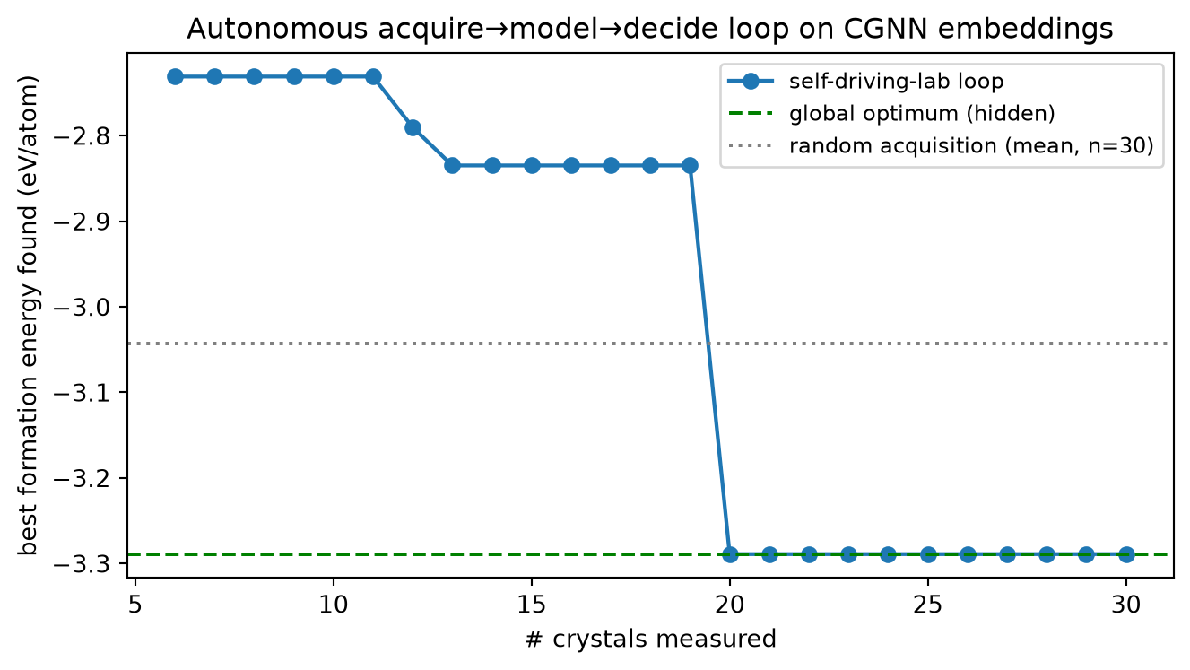
# State = frozen Block-5 trained embedding. Goal: find the most stable# (lowest formation-energy) crystal under a tight measurement budget,# without measuring all 200.emb_state = F.normalize(emb_trained, dim=1) # (200, 16) frozenenergy_oracle = y_true # "instrument": expensiveN = emb_state.shape[0]rng = np.random.default_rng(0)budget =30n_seed =5measured =list(rng.choice(N, size=n_seed, replace=False))measured = [int(i) for i in measured]best_energy_trace = []escalations =0for step inrange(budget - n_seed): idx_m = torch.tensor(measured) Zm = emb_state[idx_m] ym = energy_oracle[idx_m]# --- Model: closed-form ridge surrogate on measured crystals --- A = torch.cat([Zm, torch.ones(len(measured), 1)], dim=1) d = A.shape[1] ridge_mat =1.0* torch.eye(d); ridge_mat[-1, -1] =0.0# don't shadow the CNN regressor `reg` (used again in Block 6) w = torch.linalg.solve(A.T @ A + ridge_mat, A.T @ ym.unsqueeze(1)) resid = (A @ w).squeeze(1) - ym sigma = resid.std(unbiased=False).clamp_min(1e-3) # surrogate noise# --- Decide: acquisition over unmeasured crystals --- unmeasured = [i for i inrange(N) if i notin measured] Zu = emb_state[unmeasured] pred = (torch.cat([Zu, torch.ones(len(unmeasured), 1)], dim=1) @ w).squeeze(1)# exploration bonus: distance to the nearest measured crystal in# embedding space (far-from-known => uncertain => worth probing) nn_dist = torch.cdist(Zu, Zm).min(dim=1).values# we MINIMISE energy, so acquisition = -pred + kappa * novelty kappa =1.5 acq =-pred + kappa * nn_dist pick_local =int(acq.argmax().item()) pick = unmeasured[pick_local]# --- Escalate: conformal-style calibrated band on the surrogate ---# band half-width from the measured-residual quantile (alpha=0.1) q = torch.quantile(resid.abs(), 0.90) band =float(q.item())if band >1.5*float(sigma.item()): escalations +=1# "send to operator"# --- Acquire: reveal the true energy, add to pool --- measured.append(pick) best_energy_trace.append(float(energy_oracle[torch.tensor(measured)].min().item()))best_idx =int(energy_oracle[torch.tensor(measured)].argmin().item())best_crystal = measured[int(np.argmin([energy_oracle[m].item() for m in measured]))]global_best =float(energy_oracle.min().item())found_best = best_energy_trace[-1]print(f"Budget: {budget} measurements out of {N} crystals "f"({100*budget/N:.0f}% of the library).")print(f"Global optimum (full enumeration, NOT given to agent): "f"{global_best:+.3f} eV/atom")print(f"Best found by the loop: {found_best:+.3f} eV/atom")print(f"Operator escalations (conformal band too wide): {escalations}")# Baseline: random acquisition of the same budget, averaged over seeds.rand_best = []for s inrange(20): r = np.random.default_rng(100+ s) sample = r.choice(N, size=budget, replace=False) rand_best.append(float(energy_oracle[torch.tensor(sample)].min().item()))rand_mean =float(np.mean(rand_best))print(f"Random-acquisition baseline (same budget, mean of 20): "f"{rand_mean:+.3f} eV/atom")fig, ax = plt.subplots(figsize=(7, 4))xs =range(n_seed +1, budget +1)ax.plot(xs, best_energy_trace, "o-", lw=1.6, label="self-driving-lab loop")ax.axhline(global_best, ls="--", c="green", label="global optimum (hidden)")ax.axhline(rand_mean, ls=":", c="grey", label=f"random acquisition (mean, n={budget})")ax.set_xlabel("# crystals measured")ax.set_ylabel("best formation energy found (eV/atom)")ax.set_title("Autonomous acquire→model→decide loop on CGNN embeddings")ax.legend(fontsize=9); plt.tight_layout(); plt.show()
Budget: 30 measurements out of 200 crystals (15% of the library).
Global optimum (full enumeration, NOT given to agent): -3.289 eV/atom
Best found by the loop: -3.289 eV/atom
Operator escalations (conformal band too wide): 7
Random-acquisition baseline (same budget, mean of 20): -3.043 eV/atom
Reading the loop. The agent never sees the full library; it spends a fixed measurement budget and the active-learning acquisition (exploit the surrogate’s stability prediction, explore where the embedding is sparse) drives the best-found energy down faster than random acquisition — the self-driving-lab payoff. The conformal-style band is the deck’s automate-vs-escalate discipline: when the surrogate’s calibrated band is wide relative to its noise, the step is escalated to a human rather than silently auto-accepted. This is the same “measure, don’t assert; refuse when unsure” honesty as Block 6 — here applied to which experiment to run next instead of which sample to trust.
Why this braids cleanly. The state representation is the frozen Block-5 embedding: an embedding good enough to retrieve in (Block 5.2) is good enough to steer an autonomous experiment. MG diagnoses the representation; ML-PC puts the diagnosed representation in a closed control loop. That is the W11 triad’s actual through-line.
Block 6 — Honest limitations
Three failure modes worth seeing now, before students reach for a VAE in the wild.
Posterior collapse. Train at very high β (e.g. β = 8) and watch the KL go to zero — every encoder output collapses to the prior, and the decoder learns to ignore z entirely.
Mode collapse / lack of diversity. Sample many times at the same target energy from a CVAE that didn’t see enough training; the samples can be near-duplicates.
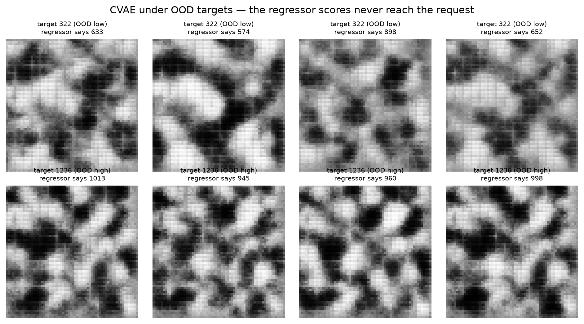
OOD targets. Ask the CVAE for an energy outside the training range; the decoder hallucinates microstructures whose predicted energy is closer to the training-range edge than to the request.
(see ML-PC §“Failure modes of inverse design”, §“Validation discipline for generative models”)
# OOD demo only (the other two are exercise material).print("OOD-target demo: ask the CVAE for energies outside training range.")y_min, y_max =float(y_tr.min()), float(y_tr.max())print(f"Training-set energy range: [{y_min:.0f}, {y_max:.0f}]")ood_low = (y_min - y_std) - y_mean # 1 std below the minood_high = (y_max + y_std) - y_mean # 1 std above the maxood_targets_n = [ood_low / y_std, ood_high / y_std]ood_labels = [f"{(ood_low+y_mean):.0f} (OOD low)", f"{(ood_high+y_mean):.0f} (OOD high)"]cvae.eval()with torch.no_grad(): fig, axes = plt.subplots(2, 4, figsize=(10, 5.5))for r, (yt, lbl) inenumerate(zip(ood_targets_n, ood_labels)): z = torch.randn(4, cvae.latent_dim, device=DEVICE) y_t = torch.full((4,), yt, device=DEVICE) samples = cvae.decode(z, y_t)# Score with the regressor. achieved = reg(samples) * y_std + y_meanfor c inrange(4): axes[r, c].imshow(samples[c, 0].cpu().numpy(), cmap="gray", vmin=0, vmax=1) axes[r, c].axis("off") axes[r, c].set_title(f"target {lbl}\nregressor says {achieved[c]:.0f}", fontsize=8)plt.suptitle("CVAE under OOD targets — the regressor scores never reach the request")plt.tight_layout(); plt.show()
OOD-target demo: ask the CVAE for energies outside training range.
Training-set energy range: [459, 1100]
Reading the OOD plot. When asked for an energy outside the training range, the CVAE produces something — but the regressor’s score on that something stays near the training-range edge. The model has no prior for samples outside its data. This is the inverse-design version of “extrapolation is not generalisation”: generative models are interpolators, not extrapolators. The discipline is to measure the achieved property (with an independent regressor) and refuse to advertise OOD candidates as valid.
Block 7 — Student exercises (~15 min)
Exercise 1 (core) — Diversity-vs-accuracy in CVAE generation
Setup. A good inverse-design generator should produce diverse candidates with the same target property. Diverse + on-target = good. Same-image-cloned + on-target = mode collapse. Different-images + off-target = bad targeting.
Task. For each of the 3 target energies in Block 2 (low / median / high), generate 20 CVAE samples. For each cohort:
Compute mean ‖regressor(sample) − y_target‖ — the accuracy.
Compute the within-cohort image-pixel variance (samples.var(dim=0).mean()) — the diversity.
Plot accuracy vs diversity for the 3 cohorts. Where on the diversity–accuracy plane does the CVAE land for each target?
Exercise 2 (core) — Latent-GD vs CVAE under OOD targets
Setup. Block 6 showed that the CVAE silently misses OOD targets. Latent-GD has a different failure mode: it can visibly diverge in loss space (you see the curve plateau or oscillate), giving a more honest “the model can’t do this” signal.
Task. Pick a target energy outside the training range (use one of ood_targets_n from Block 6). Run both methods:
CVAE: sample 8 candidates conditioned on the OOD target. Score them.
Latent-GD: run for 500 steps, plot the loss curve. Score the final z.
Report which method’s output is closer to the target, and which method’s failure signal is louder.
Exercise 3 (core) — Does pretraining actually help? The probe verdict
Setup. Block 5.1 produced a four-row probe table on a single held-out prototype (perovskite). The MG deck (§F slide 42) insists the random-init row is the comparison that decides whether training contributed or whether the architecture did the work — and it warns that a single split can mislead.
Task. Turn the single split into a verdict:
Loop over all 5 prototypes as the held-out set in turn (reuse linear_probe, emb_trained, emb_random, feat_magpie). For each fold record \(R^2\) for the trained encoder, the random-init encoder, and the Magpie-style baseline.
Report the mean ± std \(R^2\) across the 5 folds for each representation.
Answer in one sentence: on this dataset, did the supervised training of the CGNN buy a meaningful probe improvement over the random-init architecture, and does either beat the engineered Magpie-style baseline?
Expected. If trained ≈ random-init, the message-passing architecture (not the training) carries the signal — exactly the “most-omitted comparison” the deck builds §F around. If the Magpie-style row is competitive, you have measured the deck’s “always use the foundation model is wrong” claim (MG §G slide 47) on real numbers, not a slide.
Setup. The flow-matching teacher in Block 4 needs 10 ODE steps per sample (NFE = 10). A consistency model[@song_2023_consistency] distils that teacher into a one-step student\(f_\theta(x_t, t)\) that maps any point on the trajectory directly to a clean sample. The student’s training signal is consistency along the trajectory: adjacent points \((x_{t_1}, t_1)\) and \((x_{t_2}, t_2)\) on the same flow must map to the same output.
Loss. For a pair of adjacent times \(t_1 < t_2\) sampled from the trajectory of the trained teacher,
The stop-gradient on the second term turns the later student call into a fixed regression target, the way a target network is used in deep RL. After training, set \(t = 1\) at inference and sample in one forward pass (NFE = 1).
Task.
Reuse the trained flow-matching unet from Block 4 as the teacher. Build a TinyUNet student with the same architecture.
For each batch:
sample \(x_1\) from X_tr, \(x_0 \sim \mathcal{N}(0, I)\), and two times \(t_1 < t_2\) in \((0, 1)\);
form \(x_{t_1}\) and \(x_{t_2}\) on the teacher trajectory — either with the linear interpolant or, for a stronger signal, with a few Heun steps of the teacher between \(t_1\) and \(t_2\);
compute the consistency loss above and update the student.
Compare the 1-step student vs the 10-step teacher on a fresh batch of n=64 samples:
visual quality (a 4x4 grid of each);
2-Wasserstein distance between the empirical distribution of mean-pixel intensities (or any 1-D summary statistic) of the generated samples and of the data — use scipy.stats.wasserstein_distance on the 1-D summary;
Expected. The 1-step student should reach most of the teacher’s quality at 10x lower NFE — modest visual degradation but big speed-up. If the student’s W₂ distance is dramatically worse than the teacher’s, you’ve reproduced the real-world finding that one-step distillation is easy at the start of training and hard at the end (the trajectory is straighter where flow matching predicts a near-constant velocity).
Skeleton.
if HAS_GPU and unet isnotNone: teacher = unet # from Block 4for p in teacher.parameters(): p.requires_grad_(False) student = TinyUNet().to(DEVICE) opt_s = torch.optim.Adam(student.parameters(), lr=2e-4) loader_cm = DataLoader(TensorDataset(X_tr), batch_size=32, shuffle=True)for ep inrange(8):for (xb,) in loader_cm: x1 = xb; x0 = torch.randn_like(x1)# two adjacent times t1 < t2 ...# student outputs and stop-grad target ... loss = ((s1 - s2.detach()) **2).mean() opt_s.zero_grad(); loss.backward(); opt_s.step()
(see MFML §“Consistency models”; [@song_2023_consistency])
Bridge to Week 12. Next week MFML moves to uncertainty quantification (Gaussian processes, MC dropout, ensembles; the split-conformal primer was already introduced in MFML Unit 7), MG U12 turns the diagnosed embedding of this week into a generative inverse-design pipeline (MatterGen / DiffCSP / FlowMM operate on exactly the kind of representation Block 5 just verified), and ML-PC pairs both with uncertainty-aware discovery loops — the conformal escalate rule of Block 5b promoted from a guardrail to the steering signal. The discipline this week — probe before you project, measure achieved properties, refuse OOD candidates, escalate when the calibrated band is wide — is the prerequisite for honest discovery.