Week 11 — Homework (do BEFORE the Thursday exercise)

This notebook is the mandatory warm-up for the Week 11 in-class exercise. Thursday braids the three lectures materials students actually sit on 23.06 around one spine — a learned representation is only as good as what it lets you do downstream: generate, diagnose, automate. This homework primes all three so the 90 minutes can stay on the integrated story:

MFML Unit 11 — generative models. You hand-roll a VAE on Cahn–Hilliard: encoder, reparameterisation, decoder, ELBO as reconstruction + KL. This is the spine; Thursday extends it to a conditional VAE, latent-GD, and flow matching.
MG Unit 10 — Representation Learning & Feature Discovery (the true calendar-W11 MG lecture). Not latent-space arithmetic for property targeting — the W11 deck explicitly defers that to MG U12. The genuine W11 payload is embedding diagnostics: a linear probe vs a random-init baseline vs engineered features, plus nearest-neighbour retrieval, and the deck’s signature “pretty t-SNE / dead downstream” anti-pattern. You build a small guided version here so Thursday’s Block 5 can move fast.
ML-PC Unit 10 — Automation in microscopy & characterization (the true calendar-W11 ML-PC lecture). Not inverse problems — the real W11 ML-PC lecture is the self-driving lab: an autonomous acquire → model → decide loop with a conformal-style automate-vs-escalate rule. You wire a light active-learning loop stub here so Thursday’s Block 5b can go straight to the analysis.

Time: ~80 minutes.

Red thread

Week 9 read the latent space; Week 11 uses it three ways. The VAE you build (MFML) turns a latent vector \(z\) into a microstructure — a continuous knob you will steer for inverse design on Thursday. The probe stack you wire (MG) is the discipline that decides whether a learned embedding is actually doing work before you trust it. The active-learning loop you stub (ML-PC) closes the circle: an embedding good enough to retrieve in is good enough to steer an autonomous experiment.

What this homework is

Part	Min	Topic	Lecture anchor
A	25	Hand-rolled VAE on Cahn–Hilliard; ELBO = reconstruction + KL	MFML §“VAE — encoder, decoder, ELBO”, §“Reparameterisation trick”
B	18	ELBO decomposition; β-VAE sweep at β ∈ {0.1, 1.0, 4.0}	MFML §“ELBO decomposition”, §“β-VAE”
C	12	Latent-space interpolation between two CH images	MFML §“Latent traversal as a smoothness diagnostic”
D	15	(guided, runs as-is) Embedding diagnostics — linear probe vs random-init baseline	MG §F41–42 “probe before you project”, “the most-omitted comparison”
E	12	(stub, runs as-is) Self-driving-lab loop — acquire→model→decide	ML-PC §06 “Self-Driving Lab Framework”, §03 RL state/action/reward
F	8	Reflection — what does β do? what does the probe decide?	bridge to Thursday

What you must hand in (or be able to show on Thursday)

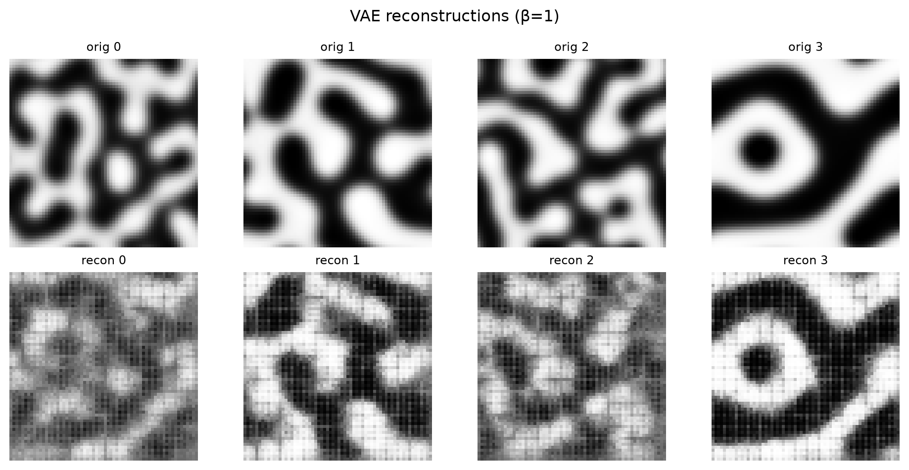
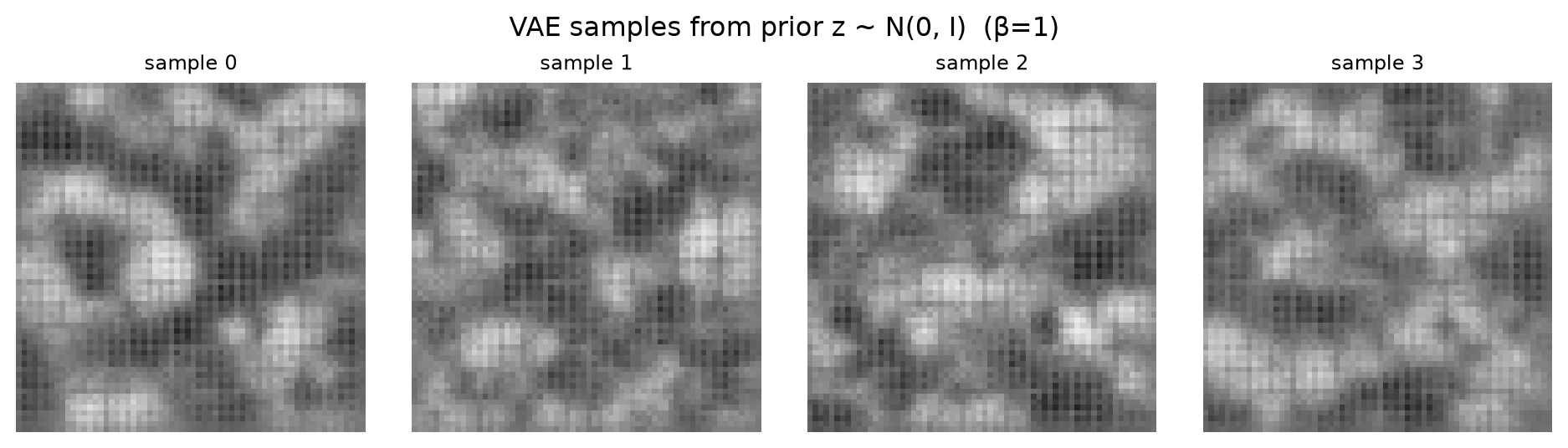
Part A: 8-image grid with 4 reconstructions and 4 prior samples; final-epoch ELBO with reconstruction term and KL term reported separately.
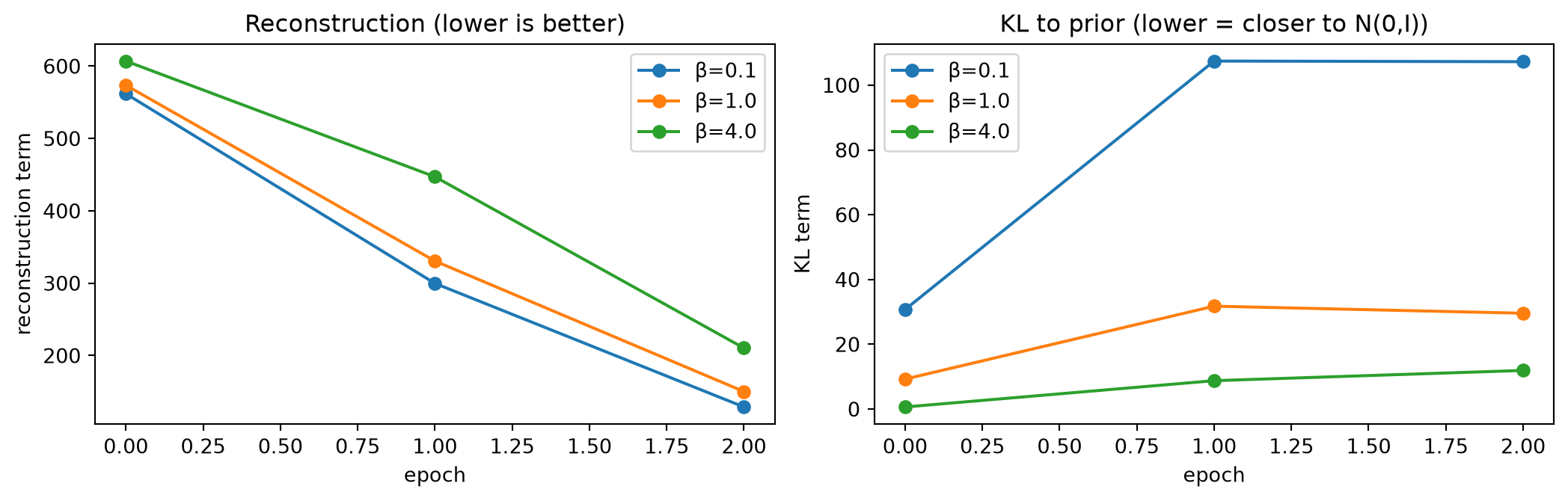
Part B: training-curve overlay of reconstruction term and KL term for the three β values.
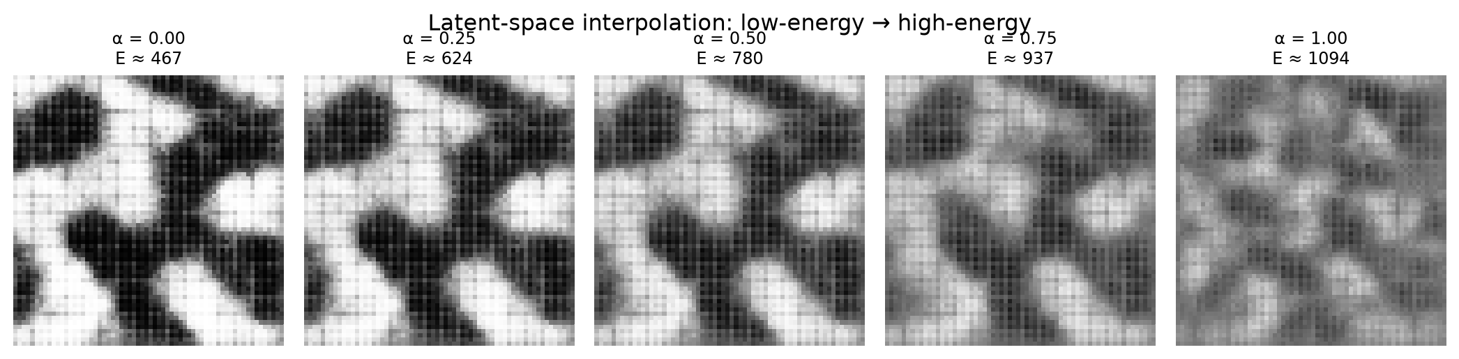
Part C: 5-image interpolation grid annotated with linearly-interpolated free energy estimates.
Part D: the completed probe table (trained encoder vs random-init vs engineered features) on a held-out prototype, with your one-line verdict on whether training (not architecture) bought anything.
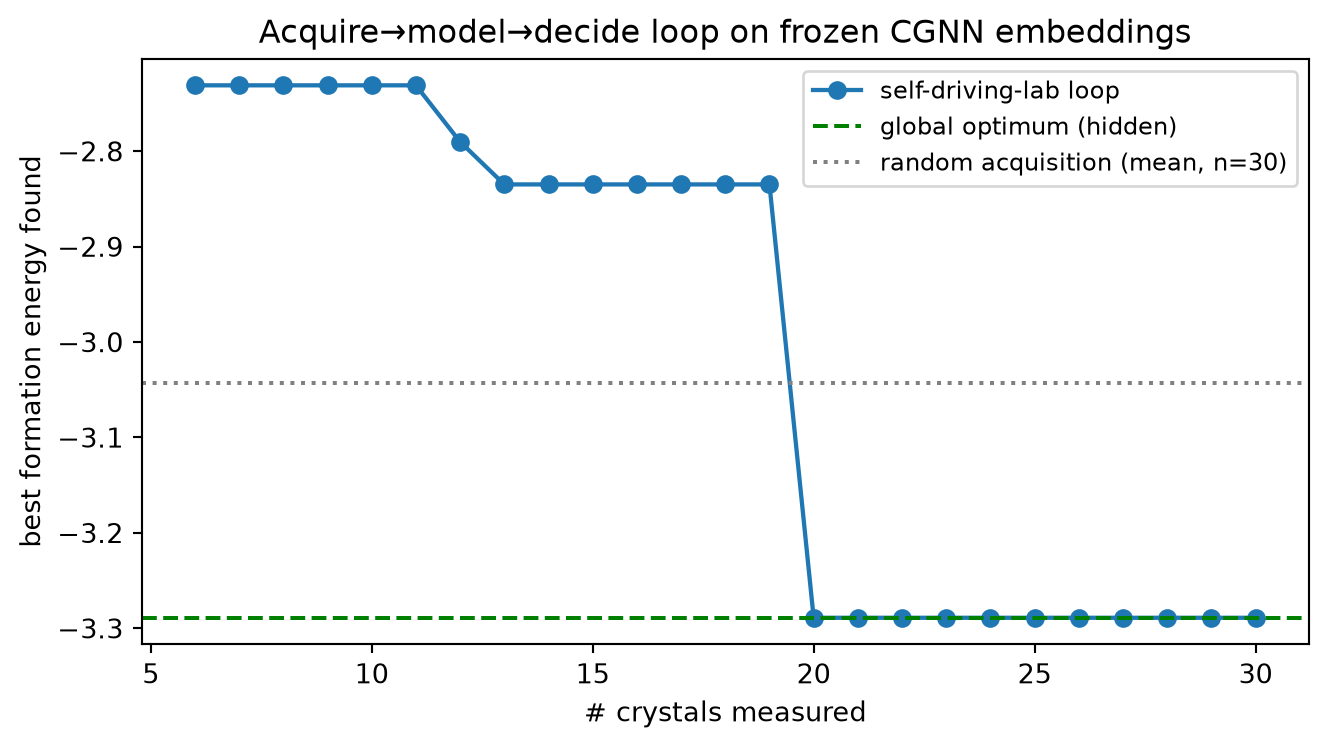
Part E: the best-energy-vs-budget curve from your acquire→model→decide loop, with the random-acquisition baseline overlaid.
Part F: paragraph (~5 sentences) on what β does + the probe verdict.

# Standard imports.  Same idiom as weeks 2-9.
import math

import numpy as np
import torch
import torch.nn as nn
import torch.nn.functional as F
from torch.utils.data import DataLoader, TensorDataset
import matplotlib.pyplot as plt

from ai4mat.datasets import CahnHilliardDataset, CrystalGraphsDataset

np.random.seed(0)
torch.manual_seed(0)

# Use GPU if available; otherwise CPU.  Everything below is device-agnostic.
DEVICE = torch.device("cuda" if torch.cuda.is_available() else "cpu")
print(f"Using device: {DEVICE}")

Using device: cpu

Helpers — load data and define the VAE

print("Loading Cahn-Hilliard (3 simulations, ~3000 samples)...")
ch = CahnHilliardDataset(simulation_number=[0, 1, 2])
print(f"  {len(ch)} samples, image shape {tuple(ch.X.shape[1:])}, "
      f"energy range = [{ch.y.min():.3g}, {ch.y.max():.3g}]")

# Standardise the energy targets for downstream use.  We will not use them
# during VAE training in Part A (the VAE is unconditional), but Part C and
# Thursday will.
y_mean = ch.y.mean().item(); y_std = ch.y.std().item()
y_norm = (ch.y - y_mean) / y_std

# Subsample for speed; 1500 train, 300 test is plenty for the VAE to learn
# basic CH structure.
g = torch.Generator().manual_seed(0)
perm = torch.randperm(len(ch), generator=g)
n_tr = 1500; n_te = 300
tr_idx, te_idx = perm[:n_tr], perm[n_tr:n_tr + n_te]
X_tr, X_te = ch.X[tr_idx].to(DEVICE), ch.X[te_idx].to(DEVICE)
y_tr_n, y_te_n = y_norm[tr_idx].to(DEVICE), y_norm[te_idx].to(DEVICE)
print(f"  train {X_tr.shape}, test {X_te.shape}")

Loading Cahn-Hilliard (3 simulations, ~3000 samples)...


  0%|          | 0/3 [00:00<?, ?it/s]
 33%|███▎      | 1/3 [00:00<00:01,  1.61it/s]
 67%|██████▋   | 2/3 [00:01<00:00,  1.94it/s]
100%|██████████| 3/3 [00:01<00:00,  1.59it/s]

  2975 samples, image shape (1, 64, 64), energy range = [458, 1.1e+03]
  train torch.Size([1500, 1, 64, 64]), test torch.Size([300, 1, 64, 64])

Part A — Hand-rolled VAE on Cahn-Hilliard

A VAE is three pieces and one trick:

Encoder \(q_\phi(z|x)\): a network that maps an image \(x\) to two vectors \(\mu(x)\) and \(\log \sigma^2(x)\) — the parameters of a diagonal Gaussian over the latent.
Reparameterisation: sample \(z = \mu + \sigma \cdot \varepsilon\) with \(\varepsilon \sim \mathcal{N}(0, I)\). The randomness is moved outside the gradient path so backprop flows through \(\mu, \sigma\).
Decoder \(p_\theta(x|z)\): a network that maps \(z\) back to a reconstructed image \(\hat x\).
ELBO loss: \[ \mathcal{L} = \underbrace{\| x - \hat x \|^2}_{\text{reconstruction}} + \underbrace{D_{\text{KL}}(q_\phi(z|x) \,\|\, p(z))}_{\text{KL to }\mathcal{N}(0,I)} \] The KL has a closed form for diagonal Gaussians: \(D_{\text{KL}} = -\tfrac{1}{2} \sum (1 + \log \sigma^2 - \mu^2 - \sigma^2)\).

(see MFML §“VAE — encoder, decoder, ELBO”, §“Reparameterisation trick”)

class TinyVAE(nn.Module):
    """64x64 grayscale -> latent_dim -> 64x64 grayscale.

    Same backbone as Week 9's conv-AE; the only changes are:
      - encoder produces 2 * latent_dim numbers (mu and log_var),
      - forward reparameterises z and returns (x_hat, mu, log_var, z).
    """

    def __init__(self, latent_dim=8):
        super().__init__()
        self.latent_dim = latent_dim
        self.enc_conv = nn.Sequential(
            nn.Conv2d(1, 16, 3, stride=2, padding=1), nn.ReLU(),    # 32x32
            nn.Conv2d(16, 32, 3, stride=2, padding=1), nn.ReLU(),   # 16x16
        )
        self.enc_lin = nn.Linear(32 * 16 * 16, 2 * latent_dim)
        self.dec_lin = nn.Linear(latent_dim, 32 * 16 * 16)
        self.dec_conv = nn.Sequential(
            nn.ConvTranspose2d(32, 16, 3, stride=2, padding=1, output_padding=1), nn.ReLU(),
            nn.ConvTranspose2d(16, 1, 3, stride=2, padding=1, output_padding=1), nn.Sigmoid(),
        )

    def encode(self, x):
        h = self.enc_conv(x).flatten(1)
        mu_logvar = self.enc_lin(h)
        return mu_logvar.chunk(2, dim=-1)                  # (mu, log_var)

    def reparameterise(self, mu, log_var):
        sigma = torch.exp(0.5 * log_var)
        eps = torch.randn_like(sigma)
        return mu + sigma * eps

    def decode(self, z):
        return self.dec_conv(self.dec_lin(z).view(-1, 32, 16, 16))

    def forward(self, x):
        mu, log_var = self.encode(x)
        z = self.reparameterise(mu, log_var)
        return self.decode(z), mu, log_var, z


def vae_loss(x, x_hat, mu, log_var, beta=1.0):
    """Sum-reduced reconstruction + beta * KL.  Returns (total, recon, kl)."""
    recon = F.mse_loss(x_hat, x, reduction="sum") / x.shape[0]
    # KL(N(mu, sigma^2) || N(0, I)) per-element, summed over latent dim.
    kl = -0.5 * (1 + log_var - mu.pow(2) - log_var.exp()).sum(dim=1).mean()
    return recon + beta * kl, recon, kl

# Train the VAE for 3 epochs at beta=1.  ~30 s on CPU, ~10 s on GPU.
def train_vae(beta, n_epochs=3, latent_dim=8, lr=1e-3, log=True):
    torch.manual_seed(0)
    model = TinyVAE(latent_dim=latent_dim).to(DEVICE)
    opt = torch.optim.Adam(model.parameters(), lr=lr)
    loader = DataLoader(TensorDataset(X_tr), batch_size=64, shuffle=True)
    rec_curve, kl_curve = [], []
    for ep in range(n_epochs):
        model.train()
        recs, kls = [], []
        for (xb,) in loader:
            x_hat, mu, log_var, _ = model(xb)
            loss, rec, kl = vae_loss(xb, x_hat, mu, log_var, beta=beta)
            opt.zero_grad(); loss.backward(); opt.step()
            recs.append(rec.item()); kls.append(kl.item())
        rec_curve.append(float(np.mean(recs)))
        kl_curve.append(float(np.mean(kls)))
        if log:
            print(f"  beta={beta:>3.1f}  epoch {ep}  recon = {rec_curve[-1]:.4f}  KL = {kl_curve[-1]:.4f}")
    return model, rec_curve, kl_curve


print("Training VAE at beta=1.0:")
vae, rec1, kl1 = train_vae(beta=1.0)

Training VAE at beta=1.0:
  beta=1.0  epoch 0  recon = 573.6272  KL = 9.2534
  beta=1.0  epoch 1  recon = 330.6285  KL = 31.7659
  beta=1.0  epoch 2  recon = 150.2331  KL = 29.5832

# Show 4 reconstructions and 4 samples from the prior.
vae.eval()
with torch.no_grad():
    x_4 = X_te[:4]
    x_hat_4, _, _, _ = vae(x_4)
    z_prior = torch.randn(4, vae.latent_dim, device=DEVICE)
    x_prior = vae.decode(z_prior)

fig, axes = plt.subplots(2, 4, figsize=(10, 5))
for i in range(4):
    axes[0, i].imshow(x_4[i, 0].cpu().numpy(), cmap="gray", vmin=0, vmax=1)
    axes[0, i].set_title(f"orig {i}", fontsize=9); axes[0, i].axis("off")
    axes[1, i].imshow(x_hat_4[i, 0].cpu().numpy(), cmap="gray", vmin=0, vmax=1)
    axes[1, i].set_title(f"recon {i}", fontsize=9); axes[1, i].axis("off")
plt.suptitle("VAE reconstructions (β=1)")
plt.tight_layout(); plt.show()

fig, axes = plt.subplots(1, 4, figsize=(10, 2.8))
for i in range(4):
    axes[i].imshow(x_prior[i, 0].cpu().numpy(), cmap="gray", vmin=0, vmax=1)
    axes[i].set_title(f"sample {i}", fontsize=9); axes[i].axis("off")
plt.suptitle("VAE samples from prior z ~ N(0, I)  (β=1)")
plt.tight_layout(); plt.show()

What you should see. Reconstructions of test images are recognisably CH-like (phase-domain texture, no stripes or salt-and-pepper noise); they are noticeably blurrier than the originals because the decoder is trying to satisfy both reconstruction and the KL pull toward \(\mathcal{N}(0, I)\). Samples from the prior are valid CH-like microstructures — fuzzier than reconstructions because the prior has no information about which mode of the CH manifold to pick.

Part B — ELBO decomposition + β-VAE sweep

β-VAE adds a single knob: the KL term gets multiplied by \(\beta\). Smaller \(\beta\) → reconstruction wins, the latent is busy and not well regularised; larger \(\beta\) → KL wins, the latent collapses toward the prior and reconstructions become bland.

We sweep \(\beta \in \{0.1, 1.0, 4.0\}\), plot the reconstruction term and KL term separately across training, and observe the trade-off.

(see MFML §“ELBO decomposition into reconstruction and KL”, §“β-VAE”)

print("\nTraining β-VAE sweep (3 betas × 3 epochs each)...")
results = {}
for beta in [0.1, 1.0, 4.0]:
    _, rec, kl = train_vae(beta=beta, log=False)
    results[beta] = (rec, kl)
    print(f"  beta = {beta:>3.1f}   final recon = {rec[-1]:.4f}   final KL = {kl[-1]:.4f}")

fig, (ax1, ax2) = plt.subplots(1, 2, figsize=(11, 3.6))
for beta, (rec, kl) in results.items():
    ax1.plot(rec, "o-", label=f"β={beta}")
    ax2.plot(kl,  "o-", label=f"β={beta}")
ax1.set_xlabel("epoch"); ax1.set_ylabel("reconstruction term"); ax1.set_title("Reconstruction (lower is better)"); ax1.legend()
ax2.set_xlabel("epoch"); ax2.set_ylabel("KL term"); ax2.set_title("KL to prior (lower = closer to N(0,I))"); ax2.legend()
plt.tight_layout(); plt.show()


Training β-VAE sweep (3 betas × 3 epochs each)...
  beta = 0.1   final recon = 128.8742   final KL = 107.2412
  beta = 1.0   final recon = 150.2331   final KL = 29.5832
  beta = 4.0   final recon = 210.3469   final KL = 11.9270

Reading the curves.

β = 0.1: reconstruction term plummets (the decoder fits the data), but the KL term is large — the latent uses much wider distributions than the prior allows. Sampling from \(\mathcal{N}(0, I)\) at this β typically misses the data manifold.
β = 1.0: the textbook setting — both terms reach an equilibrium. Reconstructions are decent and prior samples are CH-like.
β = 4.0: the KL term is small (latent is close to the prior) but reconstructions are blurry — the decoder has lost individual-sample information. This is posterior collapse.

Part C — Latent-space interpolation

A useful VAE has a smooth latent: small steps in \(z\) produce small changes in \(\hat x\). We test this by picking two test images with very different free energies, encoding both, and walking linearly between their latents.

This is a smoothness diagnostic, not yet inverse design — and note it is MFML, not MG. Latent-space arithmetic for property targeting belongs to MG U12 (Generative Models & Inverse Design); the true calendar-W11 MG lecture (Unit 10) is embedding diagnostics, which you build in Part D below.

(see MFML §“Latent traversal as a smoothness diagnostic”)

# Find a low-energy and a high-energy CH image in the test split.
y_te = ch.y[te_idx]
i_low = int(y_te.argmin().item())
i_high = int(y_te.argmax().item())
print(f"low-energy test idx = {i_low}, y = {y_te[i_low]:.3g}")
print(f"high-energy test idx = {i_high}, y = {y_te[i_high]:.3g}")

vae.eval()
with torch.no_grad():
    x_low  = X_te[i_low: i_low + 1]
    x_high = X_te[i_high: i_high + 1]
    mu_low,  _ = vae.encode(x_low)
    mu_high, _ = vae.encode(x_high)
    alphas = torch.linspace(0, 1, 5, device=DEVICE)
    interp = []
    for a in alphas:
        z = (1 - a) * mu_low + a * mu_high
        interp.append(vae.decode(z).cpu().numpy())
    grid = np.concatenate(interp, axis=0)

# Linearly interpolate the *energy* values too — to annotate the figure.
y_low  = float(y_te[i_low]); y_high = float(y_te[i_high])
y_alpha = [(1 - float(a)) * y_low + float(a) * y_high for a in alphas]

fig, axes = plt.subplots(1, 5, figsize=(11, 2.7))
for i, (a, y_a) in enumerate(zip(alphas, y_alpha)):
    axes[i].imshow(grid[i, 0], cmap="gray", vmin=0, vmax=1)
    axes[i].set_title(f"α = {float(a):.2f}\nE ≈ {y_a:.0f}", fontsize=9)
    axes[i].axis("off")
plt.suptitle("Latent-space interpolation: low-energy → high-energy")
plt.tight_layout(); plt.show()

low-energy test idx = 99, y = 467
high-energy test idx = 189, y = 1.09e+03

Reading the interpolation grid. Adjacent panels look like gradual transitions from one phase pattern to the other — that’s the smoothness we wanted from the VAE prior. Notice: the linear interpolation in energy (\(E\) on each panel) is just an annotation; the energies of the generated images are not actually the linearly-interpolated values. Verifying that “walking the latent at constant rate produces images with linearly-spaced energies” is the inverse-design question for Thursday Block 3 (latent-space gradient descent).

Part D — Embedding diagnostics (guided) — MG W11

We now leave Cahn–Hilliard images and switch to crystal embeddings, the MG home turf. The true calendar-W11 MG lecture (Unit 10, Representation Learning & Feature Discovery) is not latent-space arithmetic for property targeting — that is explicitly deferred to MG U12. Its conceptual centre is a discipline:

Probe before you project. A learned embedding is only useful to the extent it contains information about the property you care about — and a pretty 2-D projection does not establish that. The probe is the honest test; the t-SNE is the marketing image. (MG §F41.)

The single most important comparison the deck insists on (§F42) and that almost no published paper reports: the random-init baseline. A randomly-initialised encoder of the same architecture already has the architectural inductive bias (graph message passing + mean pool), just no learned weights. If a linear probe on the random-init encoder scores close to the trained encoder, then the architecture did the work and the supervised training bought little. You also compare an engineered composition baseline (a cheap Magpie-style descriptor): a learned embedding that cannot beat hand-crafted features does not justify its cost (MG §G47).

This part is guided — every cell runs as-is; three short TODO checkpoints (D.1–D.3) ask you to explain a design choice you will be quizzed on Thursday (why no optimiser on the random-init encoder; what is learned vs hand-crafted; why hold out a whole prototype). Then you read the table. Thursday’s Block 5 does the full version (retrieval, the t-SNE trap) — here you wire the spine and internalise the protocol.

(see MG §F41 “The Fundamental Diagnostic Question”, §F42 “Linear Probe Protocol — the most-omitted comparison”)

# Small graph-conv net (same backbone idea as Week 6/9): an Embedding
# table + a few message-passing layers + a regression head.  We will
# train ONE copy on toy formation energy, keep a SECOND copy at random
# init, and probe both.  (Provided in full — no TODO here.)
class TinyCGNN(nn.Module):
    def __init__(self, n_elements=120, embed_dim=16, n_layers=3):
        super().__init__()
        self.embed = nn.Embedding(n_elements, embed_dim)
        self.msg_mlps = nn.ModuleList([
            nn.Sequential(
                nn.Linear(2 * embed_dim + 1, embed_dim), nn.ReLU(),
                nn.Linear(embed_dim, embed_dim),
            ) for _ in range(n_layers)
        ])
        self.head = nn.Sequential(
            nn.Linear(embed_dim, 16), nn.ReLU(),
            nn.Linear(16, 1),
        )

    def encode(self, species, edge_index, edge_distance):
        h = self.embed(species)
        for layer in self.msg_mlps:
            src, dst = edge_index[0], edge_index[1]
            msg_in = torch.cat([h[src], h[dst], edge_distance.unsqueeze(-1)], dim=-1)
            msg = layer(msg_in)
            agg = torch.zeros_like(h).index_add_(0, dst, msg)
            h = h + agg
        return h.mean(0)                                   # mean-pooled embedding

    def forward(self, species, edge_index, edge_distance):
        return self.head(self.encode(species, edge_index, edge_distance)).squeeze(-1)


print("Loading CrystalGraphsDataset (toy formation energies)...")
cg = CrystalGraphsDataset()
y_cg = cg.y
y_cg_mean = y_cg.mean().item(); y_cg_std = y_cg.std().item()
prototype = cg.prototype
print(f"  {len(cg)} crystals, {len(cg.prototype_names)} prototypes: "
      f"{cg.prototype_names}")


def cgnn_embeddings(model):
    """Mean-pooled 16-D embedding for every crystal in `cg`. (200, 16)."""
    model.eval()
    with torch.no_grad():
        return torch.stack([
            model.encode(cg[i]["species"], cg[i]["edge_index"],
                         cg[i]["edge_distance"])
            for i in range(len(cg))
        ])


# Engineered "Magpie-style" baseline: cheap per-crystal summary stats of
# atomic number (mean, std, min, max, n_atoms).  This is the hand-crafted
# descriptor any learned embedding must BEAT to justify its cost.
def magpie_style_features():
    feats = []
    for i in range(len(cg)):
        z = cg[i]["species"].float()
        feats.append(torch.tensor([
            z.mean(), z.std(unbiased=False), z.min(), z.max(),
            float(z.numel()),
        ]))
    return torch.stack(feats)                              # (200, 5)

Loading CrystalGraphsDataset (toy formation energies)...
  200 crystals, 5 prototypes: ['rocksalt', 'zincblende', 'wurtzite', 'fluorite', 'perovskite']

# Train the supervised CGNN (this is the "pretrained" encoder).  Provided
# in full so the homework runs fast (~5 epochs, a few seconds).
torch.manual_seed(0)
cgnn = TinyCGNN()
opt_g = torch.optim.Adam(cgnn.parameters(), lr=5e-3)
print("Training TinyCGNN encoder (5 epochs, supervised on formation energy)...")
for ep in range(5):
    cgnn.train()
    losses = []
    for i in torch.randperm(len(cg)).tolist():
        s = cg[i]
        yn = (s["y"] - y_cg_mean) / y_cg_std
        opt_g.zero_grad()
        p = cgnn(s["species"], s["edge_index"], s["edge_distance"])
        loss = (p - yn) ** 2
        loss.backward()
        torch.nn.utils.clip_grad_norm_(cgnn.parameters(), 1.0)
        opt_g.step()
        losses.append(loss.item())
    if ep % 2 == 0 or ep == 4:
        print(f"  epoch {ep}  train MSE = {np.mean(losses):.4f}")

# TODO (D.1): the random-init baseline encoder is the *exact same
# architecture* as `cgnn` but NEVER trained — that is the whole point of
# the §F42 comparison.  The line below is filled so the homework runs;
# make sure you can explain *why* no optimiser is ever called on it
# (your one-sentence answer goes in Part F).
torch.manual_seed(1)
cgnn_rand = TinyCGNN()                                     # untrained on purpose

emb_trained = cgnn_embeddings(cgnn)                        # (200, 16)
# TODO (D.2): these two lines reuse the helpers above to get the
# random-init embedding and the engineered baseline.  Confirm you
# understand which one is "learned" and which is "hand-crafted".
emb_random = cgnn_embeddings(cgnn_rand)                     # (200, 16) learned-but-untrained
feat_magpie = magpie_style_features()                      # (200, 5)  hand-crafted

Training TinyCGNN encoder (5 epochs, supervised on formation energy)...
  epoch 0  train MSE = 1.0522
  epoch 2  train MSE = 0.6794
  epoch 4  train MSE = 0.4513

D.1 — Linear probe on a held-out prototype

Protocol (MG §F42). Freeze each representation. Hold out one entire prototype — evaluating a probe on the same chemistry it was fit on is a memorisation test, not a transfer test. Fit a closed-form ridge linear head on the other prototypes; report \(R^2\) / MAE on the held-out one. The linear_probe helper below is complete; you only choose the held-out prototype and read the table.

def linear_probe(Z, y, train_mask, test_mask, ridge=1.0):
    """Closed-form ridge linear probe.  Returns (R2, MAE) on the test set.

    Standardise on the train split, append a bias, solve the normal
    equations with an L2 penalty (no torch grad needed)."""
    Z = Z.float()
    mu = Z[train_mask].mean(0, keepdim=True)
    sd = Z[train_mask].std(0, keepdim=True).clamp_min(1e-6)
    Zs = (Z - mu) / sd
    Ztr = torch.cat([Zs[train_mask], torch.ones(train_mask.sum(), 1)], dim=1)
    Zte = torch.cat([Zs[test_mask], torch.ones(test_mask.sum(), 1)], dim=1)
    ytr = y[train_mask].unsqueeze(1)
    d = Ztr.shape[1]
    reg = ridge * torch.eye(d); reg[-1, -1] = 0.0          # don't penalise bias
    w = torch.linalg.solve(Ztr.T @ Ztr + reg, Ztr.T @ ytr)
    yhat = (Zte @ w).squeeze(1)
    yte = y[test_mask]
    ss_res = ((yte - yhat) ** 2).sum()
    ss_tot = ((yte - yte.mean()) ** 2).sum().clamp_min(1e-12)
    r2 = (1 - ss_res / ss_tot).item()
    mae = (yte - yhat).abs().mean().item()
    return r2, mae


# TODO (D.3): we hold out the "perovskite" prototype.  `prototype` is a
# (200,) int tensor of prototype ids.  The masks below are filled so the
# table prints; make sure you understand *why* the held-out set must be
# an entire prototype and not a random split (memorisation vs transfer —
# MG §F42).
held_out_proto = cg.prototype_names.index("perovskite")
test_mask = (prototype == held_out_proto)
train_mask = ~test_mask

print(f"Held-out prototype: 'perovskite'  "
      f"({int(test_mask.sum())} test / {int(train_mask.sum())} train)")

probe_rows = [
    ("trained CGNN encoder", emb_trained),
    ("random-init CGNN encoder", emb_random),
    ("Magpie-style features", feat_magpie),
]
print(f"\n{'representation':<28}  {'R2':>7}  {'MAE':>8}")
print("-" * 47)
for name, Z in probe_rows:
    r2, mae = linear_probe(Z, y_cg, train_mask, test_mask)
    print(f"{name:<28}  {r2:7.3f}  {mae:8.3f}")

Held-out prototype: 'perovskite'  (40 test / 160 train)

representation                     R2       MAE
-----------------------------------------------
trained CGNN encoder            0.629     0.127
random-init CGNN encoder       -0.019     0.206
Magpie-style features          -0.468     0.237

Reading the probe table (write 1 sentence for Part F). The row that matters most is random-init CGNN encoder. If it scores close to the trained encoder, the architecture did the work and the supervised training added little — exactly the “most-omitted comparison” of MG §F42. The Magpie-style row is the engineered baseline a learned embedding must beat to justify its cost. On this toy dataset formation energy is largely a composition function, so expect the cheap features to be a strong baseline — the deck’s “always use the foundation model is wrong” point, measured rather than asserted. Thursday’s Block 5 adds the retrieval check and constructs the “pretty t-SNE / dead downstream” trap on purpose; you have just wired the spine they build on.

Part E — The self-driving-lab loop (stub) — ML-PC W11

The true calendar-W11 ML-PC lecture is Unit 10 — Automation in microscopy & characterization, not inverse problems. Its spine is the self-driving lab: an agent that is given an objective (“find the most stable composition”) rather than commands, and runs an autonomous

acquire → model → decide → acquire loop

until the objective is met or the measurement budget is spent (ML-PC §06 “The Self-Driving Lab Framework”; the state/action/reward vocabulary is ML-PC §03 RL Foundations).

We make this cheap by reusing the frozen Part-D trained embedding as the lab’s state representation — closing the deck’s own forward link (“the retrieval check we run as a diagnostic becomes the operational primitive in the discovery loop”). The “instrument” is the toy formation-energy oracle cg.y; “measuring” a crystal is expensive, so the agent may only query a small budget.

Loop, one iteration:

Model. Fit a cheap ridge surrogate on everything measured so far (state = frozen embedding). (provided)
Decide. Score every unmeasured crystal with an acquisition function: exploit (predicted-low energy) + explore (distance to the nearest measured point in embedding space). (YOU fill the TODO)
Acquire. “Measure” the top-scoring crystal — reveal its true energy, add it to the labelled pool, loop. (provided)

This part is a runnable stub: the loop scaffold and a working exploit+explore acquisition rule are provided; the TODO (E.1) asks you to predict the effect of killing exploration (kappa = 0.0) and verify it. Thursday’s Block 5b adds the conformal-style automate-vs-escalate band on top of exactly this loop.

(see ML-PC §06 “Self-Driving Lab Framework”, §03 “State / Action / Reward”, §01 “objectives, not commands”)

emb_state = F.normalize(emb_trained.float(), dim=1)        # (200, 16) frozen state
energy_oracle = y_cg                                       # "instrument": expensive
N = emb_state.shape[0]

rng = np.random.default_rng(0)
budget = 30
n_seed = 5
measured = [int(i) for i in rng.choice(N, size=n_seed, replace=False)]
best_energy_trace = []

for step in range(budget - n_seed):
    idx_m = torch.tensor(measured)
    Zm = emb_state[idx_m]
    ym = energy_oracle[idx_m]

    # --- Model: closed-form ridge surrogate on measured crystals (given) ---
    A = torch.cat([Zm, torch.ones(len(measured), 1)], dim=1)
    d = A.shape[1]
    reg = 1.0 * torch.eye(d); reg[-1, -1] = 0.0
    w = torch.linalg.solve(A.T @ A + reg, A.T @ ym.unsqueeze(1))

    # --- Decide: acquisition over the unmeasured crystals ---
    unmeasured = [i for i in range(N) if i not in measured]
    Zu = emb_state[unmeasured]
    pred = (torch.cat([Zu, torch.ones(len(unmeasured), 1)], dim=1) @ w).squeeze(1)
    # exploration bonus: distance to the NEAREST measured crystal in
    # embedding space (far-from-known => uncertain => worth probing).
    nn_dist = torch.cdist(Zu, Zm).min(dim=1).values
    kappa = 1.5
    # TODO (E.1): we want the MOST STABLE crystal, i.e. we MINIMISE
    # energy.  The acquisition score below balances exploit (prefer LOW
    # predicted energy `pred`, hence the minus sign) against explore
    # (the `nn_dist` novelty bonus with weight `kappa`).  It is filled so
    # the loop runs; for Part F, predict what setting `kappa = 0.0`
    # (pure exploitation) would do to the curve, then try it.
    acq = -pred + kappa * nn_dist                          # exploit + explore
    pick = unmeasured[int(acq.argmax().item())]

    # --- Acquire: reveal the true energy, add to the pool (given) ---
    measured.append(pick)
    best_energy_trace.append(
        float(energy_oracle[torch.tensor(measured)].min().item()))

global_best = float(energy_oracle.min().item())
print(f"Budget: {budget} of {N} crystals ({100*budget/N:.0f}% of the library).")
print(f"Global optimum (full enumeration, NOT given to the agent): "
      f"{global_best:+.3f}")
print(f"Best found by the loop: {best_energy_trace[-1]:+.3f}")

# Baseline: random acquisition of the same budget, mean over 20 seeds.
rand_best = []
for s in range(20):
    r = np.random.default_rng(100 + s)
    sample = r.choice(N, size=budget, replace=False)
    rand_best.append(float(energy_oracle[torch.tensor(sample)].min().item()))
rand_mean = float(np.mean(rand_best))
print(f"Random-acquisition baseline (same budget, mean of 20): "
      f"{rand_mean:+.3f}")

fig, ax = plt.subplots(figsize=(7, 4))
xs = range(n_seed + 1, budget + 1)
ax.plot(xs, best_energy_trace, "o-", lw=1.6, label="self-driving-lab loop")
ax.axhline(global_best, ls="--", c="green", label="global optimum (hidden)")
ax.axhline(rand_mean, ls=":", c="grey",
           label=f"random acquisition (mean, n={budget})")
ax.set_xlabel("# crystals measured")
ax.set_ylabel("best formation energy found")
ax.set_title("Acquire→model→decide loop on frozen CGNN embeddings")
ax.legend(fontsize=9); plt.tight_layout(); plt.show()

Budget: 30 of 200 crystals (15% of the library).
Global optimum (full enumeration, NOT given to the agent): -3.289
Best found by the loop: -3.289
Random-acquisition baseline (same budget, mean of 20): -3.043

Reading the loop (for Part F). The agent never sees the full library; it spends a fixed measurement budget. If your acquisition rule is right, the loop’s best-found energy drops faster than random acquisition — that gap is the self-driving-lab payoff. The state it reasons over is the frozen Part-D embedding: an embedding good enough to probe/retrieve in (Part D) is good enough to steer an autonomous experiment. MG diagnoses the representation; ML-PC puts the diagnosed representation in a closed control loop. Thursday’s Block 5b adds the conformal automate-vs-escalate band — refuse to auto-accept when the calibrated band is wide — promoting this loop from a demo to a discipline.

Part F — Reflection (1 paragraph, ~5 sentences)

Write a paragraph answering both of:

(a) What does β actually control? Specifically address:

What β = 0.1 does to the latent space (use your Part B curves).
What β = 4.0 does to reconstructions (use your Part B curves and one observation from your Part C grid if you re-trained at β=4.0).
What “useful” β means for an inverse-design downstream task — do you want a sharp decoder or a well-regularised latent?

(b) What did the probe decide? In one sentence each:

From your Part D table: did the supervised training of the CGNN buy a meaningful probe improvement over the random-init architecture, and did either beat the engineered Magpie-style baseline? (This is the MG §F42 verdict in your own numbers.)
Why is the Part E loop allowed to reuse the Part D embedding as its state — i.e. what property of the embedding does Part D verify that Part E then depends on?

Bridge to Thursday. Thursday adds a condition (free energy) to the encoder/decoder — a CVAE, the simplest property-targeted generation — then a second method, latent-space gradient descent on a frozen VAE, and compares which is more honest about out-of-distribution targets. It then runs the full MG diagnostic stack (retrieval + the deliberately-constructed “pretty t-SNE / dead downstream” trap) on the embedding you just probed, and closes the ML-PC loop you stubbed with a conformal automate-vs-escalate rule. Your Part F paragraph should already have opinions about all three.

You’re done with Week 11 homework. Bring your six deliverables on Thursday:

Reconstruction grid + prior samples (Part A).
Reconstruction-vs-KL training curves at three β values (Part B).
Latent-interpolation grid with energy annotations (Part C).
Completed probe table on the held-out prototype + 1-line verdict (Part D).
Best-energy-vs-budget curve with random baseline overlaid (Part E).
Combined β + probe-verdict paragraph (Part F).

Look ahead — modern alternative to the VAE. The VAE you just built is the historical default for property-targeted generative models in materials science. The modern default for new image generators is flow matching [@lipman_2023_flow_matching]: an ODE-based generator with a simpler loss (MSE on a straight-line velocity) and ~10x fewer sampling steps than the DDPM diffusion models flow matching superseded. Thursday’s exercise notebook (week11_generative_inverse_design.py) spends Block 4 training a flow-matching model on the same Cahn–Hilliard data you just used here, so you can compare:

VAE: 1 decode call, blurry, posterior-collapse risk;
flow matching: 10 ODE steps, sharper, no posterior collapse.

An optional stretch Exercise 5 then distils the flow-matching teacher into a one-step consistency model [@song_2023_consistency] — same quality, single forward pass per sample. Worth a look if you’ve enjoyed this homework and want to see where the field has moved post-DDPM.