Week 12 — Homework (do BEFORE the Thursday exercise)
This notebook is the mandatory warm-up for the Week 12 in-class exercise. Working through it puts the GP posterior, the three predictive- uncertainty estimators (GP / MC dropout / deep ensemble), the calibration-curve diagnostic, and a first conditional generator with a discovery funnel in your hands, so Thursday can spend its 90 minutes on the harder question: how do uncertainty estimates drive a generative materials-discovery loop?
Time: ~90 minutes.
The true Week-12 triad
This week braids the true calendar-Week-12 lectures:
MFML Unit 12 — uncertainty in predictions: Gaussian Processes, MC dropout, deep ensembles, calibration (Parts A–C, the theory anchor).
ML-PC Unit 11 — materials UQ case studies: GP-for-hardness, reliability diagrams on real lab data (Part C, the lab anchor).
MG Unit 12 — Generative Models & Inverse Design: sampling structures from a learned conditional \(p(x\mid y^\star)\), conditional vs unconditional generation, classifier-free guidance, the discovery funnel, and S.U.N. (Stable/Unique/Novel) screening (Part E, the generative anchor).
Note on the MG braid (read once). Earlier drafts of this homework declared an MG lecture “clustering vs discovery in materials spaces”. That standalone clustering-as-discovery lecture was dropped in the materials_genomics realignment; old folder 11 was renamed to 12_generative_models_and_inverse_design. The true calendar-Week-12 MG lecture is therefore Unit 12: Generative Models & Inverse Design. The discovery / acquisition content you meet on Thursday is retained as the bridge into the generative half: the same GP predictive variance you build in Parts A–C becomes the “uncertainty triage” stage of the inverse-design discovery funnel (Part E).
Red thread
Materials discovery loops live or die on uncertainty: tight error bars say “exploit”, wide ones say “explore”, and an outlier without uncertainty is just noise. This week we braid Gaussian Processes (MFML), real lab case studies (ML-PC), and a conditional generative model with an inverse-design discovery funnel (MG) into an end-to-end “generate → screen → triage-by-uncertainty” materials-acceleration loop.
What this homework is
Five short workouts. Parts A–C build the UQ machinery (a GP is the minimum-friction way to put calibrated error bars on a regression model, and every other predictive-uncertainty method we use this semester is best understood as an approximation to it). Part D reflects on what an error bar means. Part E flips the arrow — from predicting a property to generating a material for a target property — and shows that the very same GP variance from Parts A–C is what decides which generated candidate is trustworthy.
Part
Min
Topic
Lecture anchor
A
25
GP regression from scratch on a 1-D toy; ML hyperparameters via L-BFGS-B
MFML §“GP posterior”, §“Hyperparameter learning”
B
20
GP vs MC dropout vs deep ensemble on the same 1-D data
MFML §“MC Dropout / Deep ensembles”
C
20
Calibration on TensileTestDataset(T=600); reliability diagram
MFML §“Calibration”; ML-PC §“Reliability diagrams on lab data”
D
10
Reflection: epistemic-uncertainty vs misspecification, with materials examples
bridge to Thursday Block 3
E
15
Conditional generator warm-up + discovery funnel with GP uncertainty triage
What you must hand in (or be able to show on Thursday)
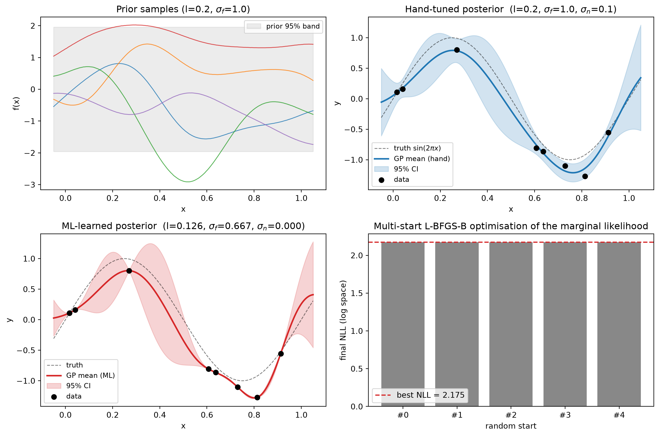
Part A: GP posterior figure showing 5 prior-sample functions, the posterior mean + 95% CI given 8 training points, and a marker at the ML-learned hyperparameters compared to the hand-tuned baseline.
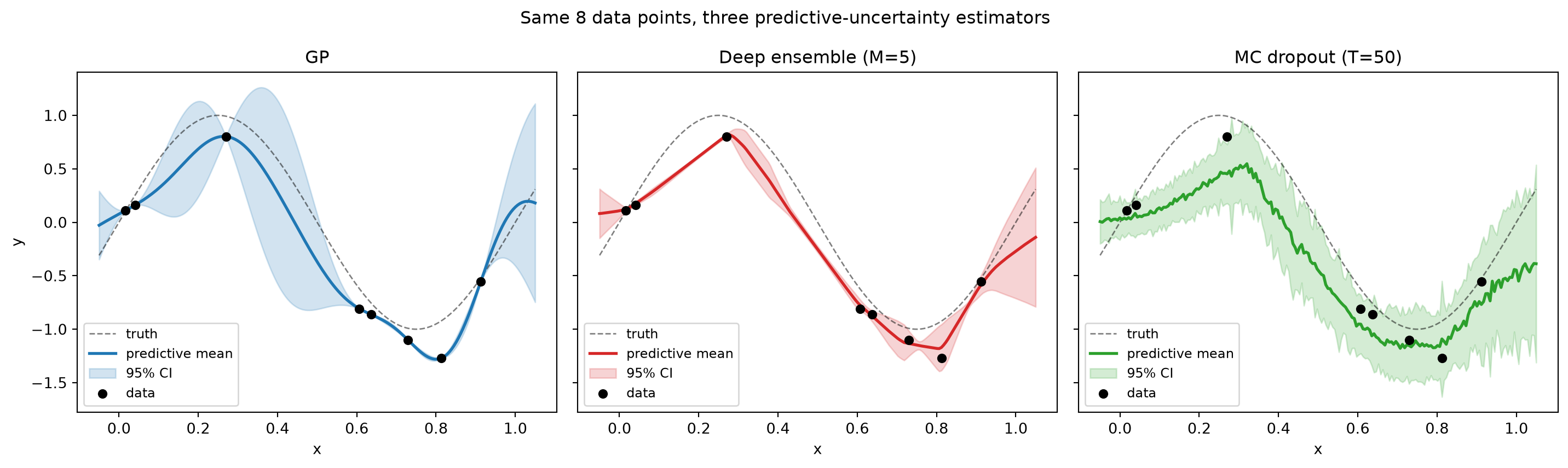
Part B: a 3-panel comparison plot (GP | MC dropout | deep ensemble) on identical data, plus the printed cost-comparison table.
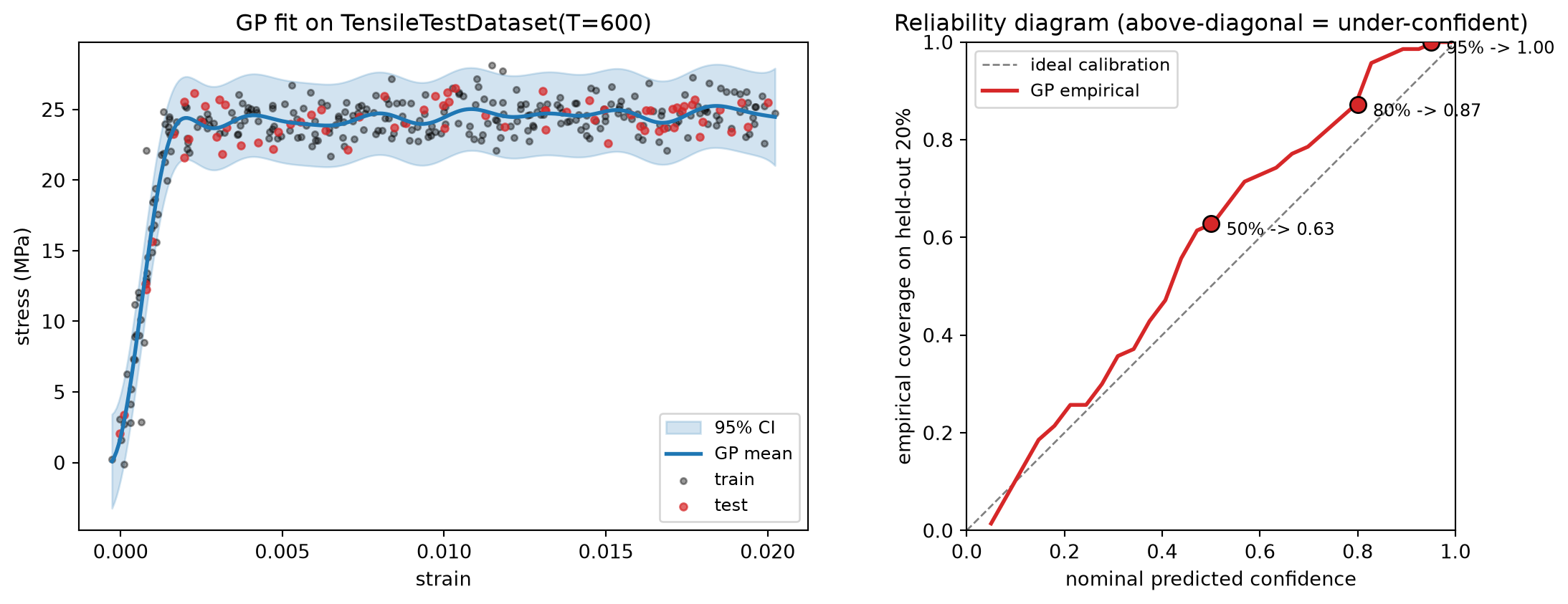
Part C: a reliability diagram (predicted-confidence vs empirical coverage) for the GP fitted on TensileTestDataset(T=600).
Part D: your written reflection paragraph (Markdown cell).
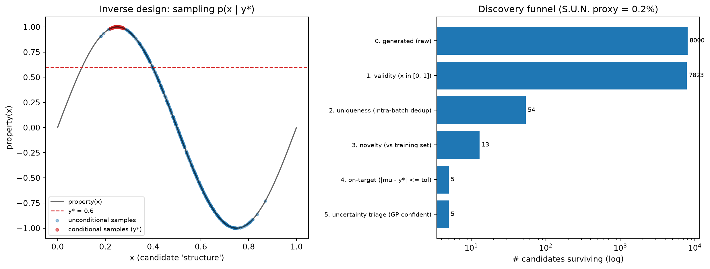
Part E: the 2-panel inverse-design figure (conditional vs unconditional samples + the discovery-funnel waterfall) and the printed funnel stage table with its S.U.N. proxy rate.
# Standard imports for the whole homework. Same idiom as weeks 2-11.import numpy as npimport torchimport torch.nn as nnimport matplotlib.pyplot as pltfrom sklearn.gaussian_process import GaussianProcessRegressorfrom sklearn.gaussian_process.kernels import RBF, WhiteKernel, ConstantKernelfrom scipy.optimize import minimizefrom scipy.stats import normfrom ai4mat.datasets import TensileTestDatasetnp.random.seed(0)torch.manual_seed(0)
<torch._C.Generator at 0x7fbdb08ce170>
Part A — GP regression from scratch on a 1-D toy
We implement a Gaussian Process regressor in NumPy in two screens of code, so the alternation between kernel (a positive-definite similarity) and posterior (a closed-form Gaussian conditional) is visible. The theory anchor is MFML §“GP posterior”:
Prior: \(f \sim \mathcal{N}(\mathbf{0}, K)\) where \(K_{ij} = k(x_i, x_j) = \sigma_f^2 \exp\!\big(-\|x_i - x_j\|^2 / (2 \ell^2)\big)\) is the squared-exponential / RBF kernel.
Three hyperparameters: lengthscale \(\ell\), signal amplitude \(\sigma_f\), noise standard deviation \(\sigma_n\). We will learn all three by maximising the log marginal likelihood.
# Generating process: y = sin(2 pi x) + 0.15 * eps, eps ~ N(0, 1).def f_true(x):return np.sin(2.0* np.pi * x)sigma_data =0.15rng = np.random.default_rng(0)N_train =8x_train = rng.uniform(0.0, 1.0, size=N_train)y_train = f_true(x_train) + sigma_data * rng.standard_normal(size=N_train)x_grid = np.linspace(-0.05, 1.05, 200)y_grid_true = f_true(x_grid)print(f"training set: N={N_train} x in [{x_train.min():.2f}, {x_train.max():.2f}] y in [{y_train.min():.2f}, {y_train.max():.2f}]")
training set: N=8 x in [0.02, 0.91] y in [-1.27, 0.80]
# Numerically stable RBF kernel and GP posterior. We add a small jitter to# the diagonal of the kernel matrix before any solve, and use np.linalg.solve# instead of np.linalg.inv (faster + better-conditioned).def rbf_kernel(X1, X2, lengthscale, sigma_f):"""Squared-exponential kernel. X1: (n1, d), X2: (n2, d).""" X1 = np.atleast_2d(X1).reshape(-1, 1) if X1.ndim ==1else X1 X2 = np.atleast_2d(X2).reshape(-1, 1) if X2.ndim ==1else X2# ||x1 - x2||^2 via the (a-b)^2 = a^2 - 2 a b + b^2 trick. sq_d = (np.sum(X1 **2, axis=1, keepdims=True)-2.0* X1 @ X2.T+ np.sum(X2 **2, axis=1)[None, :]) sq_d = np.clip(sq_d, 0.0, None)return (sigma_f **2) * np.exp(-0.5* sq_d / (lengthscale **2))def gp_posterior(x_train, y_train, x_test, lengthscale, sigma_f, sigma_n, jitter=1e-6):"""Closed-form GP posterior mean and covariance at x_test.""" K = rbf_kernel(x_train, x_train, lengthscale, sigma_f) K += (sigma_n **2+ jitter) * np.eye(len(x_train)) K_s = rbf_kernel(x_train, x_test, lengthscale, sigma_f) # (N, M) K_ss = rbf_kernel(x_test, x_test, lengthscale, sigma_f) # (M, M)# mu_* = K_s^T K^{-1} y <=> mu_* = K_s^T solve(K, y) alpha = np.linalg.solve(K, y_train) mu = K_s.T @ alpha# Sigma_* = K_** - K_s^T K^{-1} K_s v = np.linalg.solve(K, K_s) Sigma = K_ss - K_s.T @ vreturn mu, Sigma
# Sanity check: 5 sample functions from the *prior*. We sample at the test# grid x_grid by drawing from N(0, K_grid + jitter * I).lengthscale_init, sigma_f_init, sigma_n_init =0.2, 1.0, 0.1K_grid = rbf_kernel(x_grid, x_grid, lengthscale_init, sigma_f_init)K_grid +=1e-6* np.eye(len(x_grid))L_grid = np.linalg.cholesky(K_grid)prior_samples = L_grid @ rng.standard_normal(size=(len(x_grid), 5))print(f"prior samples shape: {prior_samples.shape} (length={len(x_grid)} pts, 5 functions)")
# Posterior mean + 95% CI at the *hand-tuned* hyperparameters# (lengthscale=0.2 looks reasonable for a sin curve of period 1).mu_hand, Sigma_hand = gp_posterior( x_train, y_train, x_grid, lengthscale=lengthscale_init, sigma_f=sigma_f_init, sigma_n=sigma_n_init,)sd_hand = np.sqrt(np.maximum(np.diag(Sigma_hand), 0.0))print(f"hand-tuned hyperparams: l={lengthscale_init}, sigma_f={sigma_f_init}, sigma_n={sigma_n_init}")print(f"posterior CI half-width at training points: mean = {1.96* sd_hand[::40].mean():.3f}")
hand-tuned hyperparams: l=0.2, sigma_f=1.0, sigma_n=0.1
posterior CI half-width at training points: mean = 0.361
# Negative log marginal likelihood and L-BFGS-B optimisation.## log p(y | X, theta) = -0.5 y^T (K + sigma_n^2 I)^{-1} y# - 0.5 log |K + sigma_n^2 I|# - 0.5 N log(2 pi)## We optimise in log-parameter space so the unconstrained L-BFGS-B respects# positivity. theta = [log_l, log_sigma_f, log_sigma_n].def negative_log_marginal_likelihood(theta, x, y, jitter=1e-6): log_l, log_sigma_f, log_sigma_n = theta l = np.exp(log_l); sigma_f = np.exp(log_sigma_f); sigma_n = np.exp(log_sigma_n) K = rbf_kernel(x, x, l, sigma_f) + (sigma_n **2+ jitter) * np.eye(len(x))try: L = np.linalg.cholesky(K)except np.linalg.LinAlgError:return1e8# cholesky-fail penalty alpha = np.linalg.solve(L.T, np.linalg.solve(L, y)) nll =0.5* y @ alpha + np.sum(np.log(np.diag(L))) +0.5*len(y) * np.log(2* np.pi)returnfloat(nll)# Multi-start: 5 random starts in log-space, keep the best.starts = [ np.array([np.log(0.05), np.log(0.5), np.log(0.05)]), np.array([np.log(0.20), np.log(1.0), np.log(0.10)]), np.array([np.log(0.50), np.log(2.0), np.log(0.30)]), np.array([np.log(0.10), np.log(0.3), np.log(0.20)]), np.array([np.log(1.00), np.log(1.5), np.log(0.05)]),]best =Nonefor s, theta0 inenumerate(starts): res = minimize(negative_log_marginal_likelihood, theta0, args=(x_train, y_train), method="L-BFGS-B", options=dict(maxiter=200))if best isNoneor res.fun < best.fun: best = res best_start = stheta_ml = best.xl_ml, sigma_f_ml, sigma_n_ml = np.exp(theta_ml)print(f"ML hyperparams (best of {len(starts)} starts, start #{best_start}, NLL = {best.fun:.3f}):")print(f" lengthscale = {l_ml:.4f} sigma_f = {sigma_f_ml:.4f} sigma_n = {sigma_n_ml:.4f}")
ML hyperparams (best of 5 starts, start #1, NLL = 2.175):
   lengthscale = 0.1262   sigma_f = 0.6666   sigma_n = 0.0000
# Posterior mean + 95% CI at the ML-learned hyperparameters.mu_ml, Sigma_ml = gp_posterior( x_train, y_train, x_grid, lengthscale=l_ml, sigma_f=sigma_f_ml, sigma_n=sigma_n_ml,)sd_ml = np.sqrt(np.maximum(np.diag(Sigma_ml), 0.0))
Read these four panels. The prior sample functions (top-left) are the space of all explanations the GP entertains before seeing data — wide, with no preference for any single curve. The two posterior panels show how the data collapse that prior: the ML-tuned posterior (bottom-left) tracks the truth more tightly inside the data range and has wider error bars where there is no data — exactly the qualitative behaviour we want. The NLL bar chart (bottom-right) is a small sanity check that the optimisation landscape has at least a couple of local minima; multi-start is cheap insurance.
Part A deliverable: the 4-panel figure above.
Part B — GP vs MC dropout vs deep ensemble
Three predictive-uncertainty methods on the same 1-D data:
GP (sklearn): closed-form posterior; the gold standard for small data.
Deep ensemble: train a small MLP \(M\) times with different seeds; predictive mean and standard deviation come from the empirical distribution of the \(M\) predictions.
MC dropout: train one MLP with dropout; at inference, leave dropout active and sample \(T\) stochastic forward passes (Gal & Ghahramani, 2016).
Empirical question: do the three methods produce similar error bars? Where do they disagree?
(see MFML §“MC Dropout / Deep ensembles”)
# (1) GP via sklearn (cleaner kernel API than rolling our own).kernel = ConstantKernel(1.0, (1e-3, 1e3)) * RBF(length_scale=0.2, length_scale_bounds=(1e-2, 1e1)) \+ WhiteKernel(noise_level=0.05**2, noise_level_bounds=(1e-5, 1e-1))gpr = GaussianProcessRegressor(kernel=kernel, normalize_y=True, n_restarts_optimizer=5, random_state=0)gpr.fit(x_train.reshape(-1, 1), y_train)mu_gp, sd_gp = gpr.predict(x_grid.reshape(-1, 1), return_std=True)print(f"sklearn GP fitted kernel: {gpr.kernel_}")
sklearn GP fitted kernel: 1.02**2 * RBF(length_scale=0.123) + WhiteKernel(noise_level=1e-05)
/opt/hostedtoolcache/Python/3.11.15/x64/lib/python3.11/site-packages/sklearn/gaussian_process/kernels.py:445: ConvergenceWarning: The optimal value found for dimension 0 of parameter k2__noise_level is close to the specified lower bound 1e-05. Decreasing the bound and calling fit again may find a better value.
  warnings.warn(
# Small MLP shared by the ensemble and the MC-dropout estimator.class MLP1D(nn.Module):def__init__(self, hidden=32, dropout=0.0):super().__init__()self.dropout = dropoutself.fc1 = nn.Linear(1, hidden)self.fc2 = nn.Linear(hidden, hidden)self.fc3 = nn.Linear(hidden, 1)def forward(self, x): h = torch.relu(self.fc1(x))ifself.dropout >0: h = nn.functional.dropout(h, p=self.dropout, training=True)# `training=True` forces stochastic dropout EVEN at .eval() time# -- this is the MC-dropout trick. h = torch.relu(self.fc2(h))ifself.dropout >0: h = nn.functional.dropout(h, p=self.dropout, training=True)returnself.fc3(h).squeeze(-1)def train_mlp1d(x_train, y_train, hidden=32, dropout=0.0, n_epochs=600, lr=1e-2, seed=0): torch.manual_seed(seed) model = MLP1D(hidden=hidden, dropout=dropout) opt = torch.optim.Adam(model.parameters(), lr=lr) Xt = torch.tensor(x_train.reshape(-1, 1), dtype=torch.float32) yt = torch.tensor(y_train, dtype=torch.float32)for _ inrange(n_epochs): opt.zero_grad() loss = torch.mean((model(Xt) - yt) **2) loss.backward(); opt.step()return model
# (2) Deep ensemble: train M=5 plain MLPs, no dropout, different seeds.M =5ensemble = [train_mlp1d(x_train, y_train, dropout=0.0, seed=s) for s inrange(M)]Xg = torch.tensor(x_grid.reshape(-1, 1), dtype=torch.float32)preds_ens = np.stack([m(Xg).detach().numpy() for m in ensemble], axis=0) # (M, G)mu_ens = preds_ens.mean(axis=0)sd_ens = preds_ens.std(axis=0)print(f"deep ensemble: M={M} mean SD across grid = {sd_ens.mean():.3f}")
deep ensemble: M=5 mean SD across grid = 0.057
# (3) MC dropout: train one MLP with dropout=0.2; sample T=50 forward passes.T =50mlp_dropout = train_mlp1d(x_train, y_train, dropout=0.2, seed=0)preds_mc = np.stack( [mlp_dropout(Xg).detach().numpy() for _ inrange(T)], axis=0) # (T, G)mu_mc = preds_mc.mean(axis=0)sd_mc = preds_mc.std(axis=0)print(f"MC dropout: T={T} samples mean SD across grid = {sd_mc.mean():.3f}")
MC dropout: T=50 samples mean SD across grid = 0.179
========================================================================
method               training       inference          parallelisable?
------------------------------------------------------------------------
GP                   one solve      O(N^3) once        no (sequential)
Deep ensemble        M trainings    M forwards         yes
MC dropout           one training   T forwards         yes (per pass)
========================================================================
Read this 3-panel comparison. All three methods give qualitatively similar error bars in the data-rich interior, but they differ outside it: the GP grows its CI smoothly toward the prior amplitude, the ensemble spread reflects the variability of the M MLPs (often under-confident in the interior but unpredictable in the extrapolation region), and MC dropout’s CI tracks neither cleanly — it depends heavily on the dropout rate and the number of forward passes.
Practical advice. For small data, fit a GP. For moderate data where the GP is too slow, use a deep ensemble of M=5 small MLPs. MC dropout is the cheapest of the three but the least theoretically grounded; treat its error bars as a rough heuristic rather than a calibrated estimate.
Part B deliverable: the 3-panel figure and the printed cost table.
Part C — Calibration on TensileTestDataset(T=600)
A predictive interval is calibrated if the empirical fraction of test points it covers matches the nominal level. Saying “this is my 95% interval” only means something if 95% of test points actually land inside it. We measure this on real materials data.
Recipe (MFML §“Calibration”):
Fit a GP on 80% of TensileTestDataset(T=600).
For each held-out test point, predict \((\mu_i, \sigma_i)\).
For nominal levels \(p \in \{0.50, 0.80, 0.95\}\), compute the z-multiplier \(z = \Phi^{-1}(0.5 + p / 2)\) and the empirical coverage \(\frac{1}{N}\sum_i \mathbf{1}\{|y_i - \mu_i| \le z\,\sigma_i\}\).
Plot empirical coverage vs nominal level — the diagonal is the well-calibrated line.
(see MFML §“Calibration”; ML-PC §“Reliability diagrams on lab data”)
Split-conformal primer relocated. The basic split-conformal recipe and an empirical coverage check on TensileTestDataset(T=600) now live in the Week 7 homework (week7_uncertainty_and_robustness_homework.py, Part E) [@angelopoulos_2023_conformal]. Here in Week 12 we assume you already know the recipe and exercise the more interesting variant — conformalized quantile regression (CQR) — on materials data in Thursday’s Block 4.5.
How to read a reliability diagram.
On the diagonal: the GP is well calibrated — saying “I’m 80% confident” produces an interval that contains 80% of the truth.
Above the diagonal (empirical > nominal): the GP is under-confident — its intervals are wider than necessary. Conservative; not catastrophic.
Below the diagonal (empirical < nominal): the GP is over-confident — its intervals are too narrow. Dangerous: a “95% CI” that covers 70% of test points means you will under-estimate experimental risk.
Take-away. Calibration is a property of the model on this data, not of the GP framework in general. A GP with a misspecified kernel (too short a lengthscale, wrong noise scale) is just as miscalibrated as any other model. Always plot a reliability diagram before shipping a UQ-driven decision pipeline — Block 5 of Thursday’s notebook will return to this.
Part C deliverable: the right-hand panel of the figure above.
Part D — Reflection: epistemic vs misspecification
A wide error bar can mean one of two very different things:
Epistemic uncertainty. The model knows the data does not constrain its prediction here — the right fix is more data (active learning, additional experiments). The GP’s CI grows in extrapolation regions for exactly this reason.
Model misspecification. The model is wrong (wrong kernel, wrong likelihood, wrong feature representation). More data does not help; in fact it can hurt by sharpening a wrong belief. The fix is to change the model.
Reliability diagrams (Part C) hint at which one you have: a model that is systematically over-confident is usually misspecified, while a model whose CI grows where expected (sparse data, edges of strain support) is usually epistemically uncertain in the right way.
Your task (~10 min, write 5–8 sentences):
Give a concrete materials-science example where wide error bars legitimately mean “the model knows it doesn’t know” and adding experiments would close them. (Hint: think hardness measurements at a Cr-content the calibration set never covered.)
Give a concrete materials-science example where wide error bars are a misspecification artefact — adding experiments would not fix them. (Hint: think GP with an RBF kernel on a piecewise-linear yield-surface response, or a stationary kernel where the noise is actually heteroscedastic.)
Bring this paragraph to Thursday; we will pick two volunteers to read theirs aloud at the start of Block 1, and Block 3’s cost-aware AL loop will revisit your answer with measurements.
Hand in: your written paragraph (Markdown cell below).
Your answer:
(replace this text with your paragraph)
Part E — Inverse design warm-up: a conditional generator + discovery funnel
Parts A–D were all forward: given an input, predict a property and its uncertainty. MG Unit 12 (Generative Models & Inverse Design) inverts the arrow. Instead of searching a materials space we sample from a learned conditional distribution\(p(x \mid y^\star)\): name a target property \(y^\star\), get a stream of candidate materials.
Real crystal generators (the deck’s CDVAE → DiffCSP → MatterGen → FlowMM → CrystaLLM lineage) denoise/flow over composition + lattice + coordinates + space group with equivariant GNNs at O(100) network passes per sample. That is far out of scope for a homework cell. We build the tractable 1-D teaching analogue the deck itself motivates — a tiny conditional VAE (CVAE), the “legacy VAE row” of the deck’s landscape table. The conditional-sampling, classifier-free-guidance, and discovery-funnel logic are structurally identical to the SOTA models; only the decoder changes. On Thursday (Block 6.5) you scale exactly this to the 2-D NanoindentationDataset (E, H) analogue.
You will exercise four things the deck teaches, in order:
A learned \(p(x \mid y^\star)\) — train the CVAE on a 1-D toy where the property is a known function of \(x\), then generate candidates conditioned on a target.
Conditional vs unconditional generation + classifier-free guidance (CFG) — the deck’s \(\tilde s = (1+w)\,s_{\text{cond}} -
w\,s_{\text{uncond}}\) knob has an exact CVAE analogue.
The discovery funnel + S.U.N. — push generated candidates through validity → uniqueness → novelty → on-target → uncertainty triage and report the surviving fraction at every stage.
Uncertainty-aware filtering = the generative↔︎UQ bridge — the triage stage reuses a GP predictive variance (exactly the Part A/C machinery): reject candidates the surrogate cannot vouch for.
(see MG U12 §“Forward vs Inverse Problems”, §“Conditional vs Unconditional Generation”, §“Classifier vs Classifier-Free Guidance”, §“The Discovery Funnel”, §“The S.U.N. Metric”, §“Uncertainty-Aware Filtering”; bridges to MFML §“GP posterior” and ML-PC §“GP for hardness”.)
# A 1-D inverse-design toy. The "structure" is a scalar x in [0, 1]; the# "property" is y = property(x) = sin(2 pi x) (the same generative process# as Part A, so the GP you already trust is the surrogate). Inverse design:# given a target property y*, find x with property(x) ~= y*. This is# deliberately *many-to-one* (sin hits most levels twice on [0, 1]) and has# no closed-form inverse — the deck's "inverse is ill-posed" point in 1-D.def property_fn(x):return np.sin(2.0* np.pi * x)rng_e = np.random.default_rng(0)N_pool =600x_pool = rng_e.uniform(0.0, 1.0, size=N_pool).astype(np.float32)y_pool = property_fn(x_pool).astype(np.float32)print(f"inverse-design pool: N={N_pool} x in [0, 1] "f"property in [{y_pool.min():.2f}, {y_pool.max():.2f}]")
inverse-design pool: N=600 x in [0, 1] property in [-1.00, 1.00]
# A deliberately tiny conditional VAE: 1-D data, 1-D latent, 1-D# conditioner (the target property). Same torch idiom as the MLP1D in# Part B. The encoder sees (x, c); the decoder sees (z, c).## CFG hook (deck §"Classifier-free guidance"): during training we randomly# *drop* the conditioning signal (replace c by a null token = 0) with# probability p_drop, so the SAME weights learn both a conditional and an# unconditional model — the precondition CFG needs.class CVAE1D(nn.Module):def__init__(self, hidden=32, z_dim=2):super().__init__()self.z_dim = z_dimself.enc = nn.Sequential( nn.Linear(1+1, hidden), nn.ReLU(), nn.Linear(hidden, hidden), nn.ReLU(), )self.fc_mu = nn.Linear(hidden, z_dim)self.fc_lv = nn.Linear(hidden, z_dim)self.dec = nn.Sequential( nn.Linear(z_dim +1, hidden), nn.ReLU(), nn.Linear(hidden, hidden), nn.ReLU(), nn.Linear(hidden, 1), )def encode(self, x, c): h =self.enc(torch.cat([x, c], dim=1))returnself.fc_mu(h), self.fc_lv(h)def reparameterise(self, mu, logvar): std = torch.exp(0.5* logvar)return mu + std * torch.randn_like(std)def decode(self, z, c):returnself.dec(torch.cat([z, c], dim=1))def forward(self, x, c): mu, lv =self.encode(x, c) z =self.reparameterise(mu, lv)returnself.decode(z, c), mu, lv
# Train the CVAE. Standard VAE ELBO = reconstruction (MSE) + beta * KL,# with the CFG conditioning-dropout above. Tiny model, CPU, a few seconds.## TODO (E.1): the two ELBO terms below are written out in full so the# notebook runs end-to-end out of the box. BEFORE looking at them, cover# the two lines and re-derive them yourself: (a) the reconstruction term is# the per-sample squared error summed over the data dim and averaged over# the batch; (b) the KL of a diagonal-Gaussian posterior N(mu, sigma^2)# against the N(0, I) prior is KL = -0.5 * sum(1 + log sigma^2 - mu^2 -# sigma^2). Confirm your hand-derived expressions match the code.torch.manual_seed(0)cvae = CVAE1D(hidden=32, z_dim=2)opt_v = torch.optim.Adam(cvae.parameters(), lr=5e-3)x_t = torch.tensor(x_pool.reshape(-1, 1), dtype=torch.float32)c_t = torch.tensor(y_pool.reshape(-1, 1), dtype=torch.float32) # condition on the propertyNe = x_t.shape[0]beta_kl =0.1# mild KL pressure: enough to keep the latent# sample-able, low enough that the decoder still# *uses* z (avoid posterior collapse -> diversity)p_drop =0.15# CFG conditioning-dropout probabilitybatch_e =128rng_t = np.random.default_rng(0)for epoch inrange(150): order = rng_t.permutation(Ne) epoch_loss =0.0for s inrange(0, Ne, batch_e): idx = order[s:s + batch_e] xb = x_t[idx] cb = c_t[idx].clone() drop = torch.rand(cb.shape[0]) < p_drop # CFG: drop the label cb[drop] =0.0# null token xr, mu_z, lv_z = cvae(xb, cb)# (E.1a) reconstruction term: per-sample squared error, summed over# the data dim, averaged over the batch. rec = ((xr - xb) **2).sum(dim=1).mean()# (E.1b) KL of the diagonal-Gaussian posterior vs the N(0, I) prior# (lv_z is log sigma^2), averaged over the batch. kl = (-0.5* (1+ lv_z - mu_z.pow(2) - lv_z.exp()).sum(dim=1)).mean() loss = rec + beta_kl * kl opt_v.zero_grad(); loss.backward(); opt_v.step() epoch_loss +=float(loss) *len(idx)if epoch %50==0or epoch ==149:print(f"epoch {epoch:3d} ELBO loss = {epoch_loss / Ne:.4f}")
epoch 0 ELBO loss = 0.2002
/tmp/ipykernel_4165/1967593832.py:44: UserWarning: Converting a tensor with requires_grad=True to a scalar may lead to unexpected behavior.
Consider using tensor.detach() first. (Triggered internally at /pytorch/torch/csrc/autograd/generated/python_variable_methods.cpp:838.)
  epoch_loss += float(loss) * len(idx)
epoch  50   ELBO loss = 0.0352
epoch 100   ELBO loss = 0.0342
epoch 149   ELBO loss = 0.0296
# ---- Generation: sample from p(x | y*) with classifier-free guidance ----## CFG analogue for a CVAE decoder. Pure conditional decode = decode(z, c*).# Pure unconditional decode = decode(z, 0 (null)). The deck mixes the# conditional and unconditional *scores*; for a deterministic decoder the# standard analogue extrapolates the decoded value along the# (conditional - unconditional) direction:## x_cfg = x_uncond + (1 + w) * (x_cond - x_uncond)## w = 0 -> plain conditional; w > 0 -> push further along the "conditioning# made a difference" direction. The deck warns the guidance strength is "a# constant battle": too little ignores the target, too much overshoots and# kills diversity. You will see both regimes.def generate(model, y_target, n_samples, guidance_w=0.0, seed=0):"""Sample n_samples candidate x conditioned on a target property y*.""" torch.manual_seed(seed) c_star = torch.full((n_samples, 1), float(y_target)) c_null = torch.zeros((n_samples, 1)) z = torch.randn(n_samples, model.z_dim)with torch.no_grad(): x_cond = model.decode(z, c_star)if guidance_w ==0.0: x_gen = x_condelse: x_uncond = model.decode(z, c_null) x_gen = x_uncond + (1.0+ guidance_w) * (x_cond - x_uncond)return x_gen.numpy().ravel()# Target on the upper half of the property range — an "I want a material# with property ~= 0.6" inverse-design ask.Y_STAR =0.6print(f"inverse-design target: y* = {Y_STAR:.2f}")for w in (0.0, 0.5, 1.5, 4.0): g = generate(cvae, Y_STAR, n_samples=400, guidance_w=w, seed=1) g = np.clip(g, 0.0, 1.0) prop_err = np.abs(property_fn(g) - Y_STAR)print(f" CFG w={w:>3.1f}: mean |property(x_gen) - y*| = {prop_err.mean():.3f}"f" x_gen spread (std) = {g.std():.3f}")print(" (w=0 collapses onto ONE narrow mode; turning guidance up widens"" the stream so it covers more of the valid pre-image set, at the"" cost of per-sample fidelity — the deck's fidelity<->diversity"" trade-off, in 1-D.)")
inverse-design target: y* = 0.60
  CFG w=0.0:  mean |property(x_gen) - y*| = 0.398   x_gen spread (std) = 0.011
  CFG w=0.5:  mean |property(x_gen) - y*| = 0.256   x_gen spread (std) = 0.066
  CFG w=1.5:  mean |property(x_gen) - y*| = 0.529   x_gen spread (std) = 0.065
  CFG w=4.0:  mean |property(x_gen) - y*| = 0.571   x_gen spread (std) = 0.059
  (w=0 collapses onto ONE narrow mode; turning guidance up widens the stream so it covers more of the valid pre-image set, at the cost of per-sample fidelity — the deck's fidelity<->diversity trade-off, in 1-D.)
# A reusable GP surrogate for the property — this is the *exact same*# sklearn-GP recipe you used in Parts B and C. Its predictive standard# deviation is the "uncertainty triage" knob of the funnel below.kernel_e = ConstantKernel(1.0, (1e-3, 1e3)) \* RBF(length_scale=0.15, length_scale_bounds=(1e-2, 1e0)) \+ WhiteKernel(noise_level=0.05**2, noise_level_bounds=(1e-5, 1e-1))gp_surrogate = GaussianProcessRegressor(kernel=kernel_e, normalize_y=True, n_restarts_optimizer=3, random_state=0)# Train the surrogate on a SUBSET (first 60 pool points) so it is# legitimately *uncertain* away from where it has seen data — that is what# makes the triage stage do real work.n_surr =60gp_surrogate.fit(x_pool[:n_surr].reshape(-1, 1), y_pool[:n_surr])print(f"surrogate GP trained on {n_surr} points; kernel = {gp_surrogate.kernel_}")
surrogate GP trained on 60 points; kernel = 2.13**2 * RBF(length_scale=0.382) + WhiteKernel(noise_level=1e-05)
/opt/hostedtoolcache/Python/3.11.15/x64/lib/python3.11/site-packages/sklearn/gaussian_process/kernels.py:445: ConvergenceWarning: The optimal value found for dimension 0 of parameter k2__noise_level is close to the specified lower bound 1e-05. Decreasing the bound and calling fit again may find a better value.
  warnings.warn(
# ---- The discovery funnel + S.U.N.-style screening ----## Deck §"The Discovery Funnel" / §"The S.U.N. Metric": a generated stream# is only useful after a multi-stage filter, each stage trimming ~10-100x.# We instantiate the deck's funnel on the 1-D analogue:## generate (wide top) -> raw candidates# -> VALIDITY : physically plausible (x in [0, 1])# -> UNIQUENESS within batch : de-duplicate near-identical samples# -> NOVELTY vs training set : far from any pool point already seen# -> ON-TARGET (fidelity) : |property(x) - y*| within tolerance# -> UNCERTAINTY TRIAGE : the surrogate GP must be *confident*# (predictive sd below a cutoff) — the# generative <-> UQ bridge## "S.U.N." = Stable . Unique . Novel; we report the fraction of the raw# batch surviving the U+N stages, plus the final end-to-end yield.def discovery_funnel(cand_x, y_target, gp, x_known, novelty_tol=0.01, target_tol=0.15, gp_sd_cutoff=0.20, verbose=True):"""Run the multi-stage funnel; return survivors + a stage table.""" stages = [] x = np.asarray(cand_x, dtype=np.float64).ravel() stages.append(("0. generated (raw)", len(x)))# --- VALIDITY: in the physical [0, 1] range. x = x[(x >=0.0) & (x <=1.0)] stages.append(("1. validity (x in [0, 1])", len(x)))# --- UNIQUENESS: grid-snap, drop duplicates.iflen(x): keys = np.round(x /0.005).astype(np.int64) _, uniq_idx = np.unique(keys, return_index=True) x = x[np.sort(uniq_idx)] stages.append(("2. uniqueness (intra-batch dedup)", len(x)))# --- NOVELTY: far enough from every training point.iflen(x): d = np.abs(x[:, None] - x_known[None, :]).min(axis=1) x = x[d > novelty_tol] stages.append(("3. novelty (vs training set)", len(x))) sun_rate =len(x) /max(stages[0][1], 1)# --- ON-TARGET: predicted property close to the conditioning target.# Use the GP MEAN as the property predictor (we do not get to call# the true property_fn in a real campaign — only the surrogate).iflen(x): mu_pred, sd_pred = gp.predict(x.reshape(-1, 1), return_std=True) on_target = np.abs(mu_pred - y_target) <= target_tol x, sd_pred = x[on_target], sd_pred[on_target] stages.append(("4. on-target (|mu - y*| <= tol)", len(x)))# --- UNCERTAINTY TRIAGE: keep only candidates the surrogate is# confident about (predictive sd below the cutoff). This is the# Part A/C GP variance deciding which generated candidate to trust.iflen(x): confident = sd_pred <= gp_sd_cutoff x = x[confident] stages.append(("5. uncertainty triage (GP confident)", len(x)))if verbose:print(f" {'stage':<42s}{'#kept':>7s}{'frac':>9s}") n0 =max(stages[0][1], 1)for name, n in stages:print(f" {name:<42s}{n:>7d}{n / n0:>8.1%}")print(f" S.U.N. rate (Stable*Unique*Novel proxy) = {sun_rate:.1%}")print(f" end-to-end discovery yield = {len(x) / n0:.1%}")return x, stages, sun_rate# Wide top of funnel: over-generate, exactly as the deck insists. Light# guidance (w=0.5) refines toward y* without overshooting.raw = generate(cvae, Y_STAR, n_samples=8000, guidance_w=0.5, seed=7)survivors, stage_table, sun = discovery_funnel( raw, Y_STAR, gp_surrogate, x_pool[:n_surr])
# Deliverable: (left) conditional vs unconditional samples on the property# curve; (right) the funnel waterfall.g_uncond = generate(cvae, 0.0, n_samples=400, guidance_w=0.0, seed=2)g_cond = generate(cvae, Y_STAR, n_samples=400, guidance_w=0.0, seed=3)g_uncond = np.clip(g_uncond, 0.0, 1.0)g_cond = np.clip(g_cond, 0.0, 1.0)fig, axes = plt.subplots(1, 2, figsize=(13, 5.0))ax = axes[0]xs = np.linspace(0.0, 1.0, 300)ax.plot(xs, property_fn(xs), "k-", lw=1.5, alpha=0.6, label="property(x)")ax.axhline(Y_STAR, color="#d62728", ls="--", lw=1.2, label=f"y* = {Y_STAR}")ax.scatter(g_uncond, property_fn(g_uncond), c="#1f77b4", s=12, alpha=0.4, label="unconditional samples")ax.scatter(g_cond, property_fn(g_cond), c="#d62728", s=14, alpha=0.6, label="conditional samples (y*)")ax.set_xlabel("x (candidate 'structure')")ax.set_ylabel("property(x)")ax.set_title("Inverse design: sampling p(x | y*)")ax.legend(fontsize=8, loc="lower left")ax = axes[1]labels = [s[0] for s in stage_table]counts = [s[1] for s in stage_table]ax.barh(range(len(counts)), np.maximum(counts, 1), color="#1f77b4")ax.set_yticks(range(len(labels)))ax.set_yticklabels(labels, fontsize=8)ax.invert_yaxis()ax.set_xscale("log")ax.set_xlabel("# candidates surviving (log)")ax.set_title(f"Discovery funnel (S.U.N. proxy = {sun:.1%})")for i, c inenumerate(counts): ax.text(max(c, 1), i, f" {c}", va="center", fontsize=8)plt.tight_layout()plt.show()
Read these two panels. Left: unconditional samples (blue) scatter over the whole curve; conditioning on \(y^\star\) (red) pulls the stream onto the requested property band — sample from p(x \mid y^\star) made concrete. Note inverse design is many-to-one: \(\sin\) hits \(y^\star=0.6\) at two distinct \(x\) values; the plain conditional sample tends to collapse onto one pre-image (the printed CFG sweep above shows the low-spread \(w=0\) mode), and dialing classifier-free guidance up widens coverage toward the other valid branch at the cost of per-sample fidelity — the deck’s exact fidelity↔︎diversity warning. Right: the deck’s funnel made literal — each stage trims the stream (log axis); the wide top is mandatory because the end-to-end yield is a small fraction, which is why real pipelines over-generate by \(10^5\)–\(10^6\).
The braid, stated plainly. The uncertainty-triage stage is not a new idea bolted on: it is literally a GP predictive variance (the Part A/C machinery, the ML-PC GP-for-hardness story) deciding which generated (MG) candidate is trustworthy enough to act on. Generation proposes; uncertainty disposes. On Thursday (Block 6.5) you swap this 1-D toy for the 2-D NanoindentationDataset (E, H) CVAE and the funnel’s triage stage becomes the Block-5 per-cluster GP — same logic, one dimension up.
Honest caveats. (1) A 1-D CVAE is a teaching analogue: real crystal generators sample (composition, lattice, coordinates, space group) with equivariant denoisers (CDVAE → DiffCSP → MatterGen → FlowMM), but the conditional-sampling, CFG, and funnel logic are structurally identical. (2) Our “stability” proxy is in-range validity, not an energy-above-hull computation; the deck is explicit that real S.U.N. depends on the reference convex hull. (3) The novelty/target/uncertainty thresholds are policy choices — Thursday’s Exercise 6 sweeps the guidance weight and the funnel cutoffs so you feel the yield/quality trade-off.
Part E reflection (~5 min, write 3–4 sentences in the cell below).
Raise gp_sd_cutoff from 0.20 toward a large value (e.g. 1e3) and re-run the funnel cell. Which stage’s survivor count changes, and what does “turning off uncertainty triage” do to the quality of the surviving candidates (not just their count)?
In one sentence: why is it dangerous to ship the on-target survivors without the triage stage, given what Part D taught you about epistemic uncertainty vs misspecification?
Your Part E answer:
(replace this text with your 3–4 sentences)
Part E+ (optional stretch) — the same funnel on REAL crystals
The 1-D toy above isolated the mechanics. This optional stretch shows the same funnel transfers verbatim to real crystals: the perovskite subset (perov_5) of the CDVAE benchmark (Xie et al., ICLR 2022) — the dataset family the deck’s CDVAE→DiffCSP→MatterGen→FlowMM lineage is trained on. Each material is a 118-dim composition (element-fraction) vector with a scalar DFT property; no CVAE rebuild — you screen a candidate stream with the deck’s funnel, ensemble-variance doing the uncertainty triage (Thursday’s Block 6.5 Stage B does exactly this).
This is scaffolded as TODOs: fill the four marked lines, then run.
# TODO (E.2): load the real CDVAE perovskite set and DISCOVER its numeric# target column at runtime (do NOT hard-code a column name — the loader's# numeric columns differ per subset). Skeleton:## from ai4mat.datasets import CDVAEMaterialsDataset# import numpy as np# from sklearn.ensemble import RandomForestRegressor## ds_cd = CDVAEMaterialsDataset(subset="perov_5", split="train",# root="data/cdvae", download=True)# # the loader resolves a valid per-subset default for you:# target_col = ds_cd.target# numeric_cols = [c for c in ds_cd.df.columns# if np.issubdtype(ds_cd.df[c].dtype, np.number)# and c != "material_id"]# print("numeric columns:", numeric_cols, "| target =", target_col)## N = min(6000, ds_cd.X.shape[0])# X_cd = ds_cd.X.numpy()[:N].astype(np.float64) # (N, 118) compositions# y_cd = ds_cd.y.numpy()[:N].astype(np.float64) # (N,) real DFT property## TODO (E.3): fit a small random-forest surrogate on a 60% split; the mean# of the trees is the property prediction, the cross-tree std is the# epistemic-uncertainty estimate (the deck's "ensemble variance"# alternative to the GP for the uncertainty-triage stage). Skeleton:## rng = np.random.default_rng(0); perm = rng.permutation(N)# tr, ho = perm[:int(0.6 * N)], perm[int(0.6 * N):]# rf = RandomForestRegressor(n_estimators=120, max_depth=12,# n_jobs=-1, random_state=0).fit(X_cd[tr], y_cd[tr])# def rf_mu_sd(X):# P = np.stack([t.predict(X) for t in rf.estimators_], 0)# return P.mean(0), P.std(0)## TODO (E.4): emulate a generator's OUTPUT stream (no 118-dim CVAE) by# multiplicative composition-space jitter of the disjoint hold-out# crystals, renormalised to sum to 1; target the 75th-pct property.# Skeleton:## def emulate(X_seed, n, jitter=0.15, seed=7):# g = np.random.default_rng(seed)# c = X_seed[g.integers(0, len(X_seed), n)].copy()# c = np.clip(c * g.gamma(1.0 / jitter, size=c.shape), 0, None)# r = c.sum(1, keepdims=True); r[r == 0] = 1.0# return c / r# X_seed = X_cd[ho]; y_star = float(np.percentile(y_cd, 75))# raw = emulate(X_seed, 8000)## TODO (E.5): run the SAME six-stage funnel as the 1-D `discovery_funnel`# above, adapted to compositions — validity (non-negative, sums to ~1),# intra-batch uniqueness (round + dedup), novelty (min L1 distance to# X_seed > ~0.20), on-target (|rf-mean - y_star| <= rf hold-out MAE),# uncertainty triage (cross-tree sd <= 60th-pct of sd on X_seed). Print# the stage table + S.U.N. rate, and barh the waterfall on a log x-axis.# The waterfall must be NON-degenerate (survivors > 0, but a small# fraction of the raw batch) — the deck's "wide top is mandatory" picture# on real data. Reflect (2 sentences): how does the real-crystal yield# compare to the 1-D toy's, and why is the validity stage so much harder# in 118-dim composition space than in 1-D [0, 1]?
Your Part E+ reflection (optional):
(2 sentences: real-crystal yield vs 1-D toy; why 118-dim validity is harder)
Hand-in checklist
Bring (or have on screen) the following on Thursday:
The 4-panel GP-from-scratch figure from Part A (prior samples, hand- tuned posterior, ML-tuned posterior, NLL multi-start).
The 3-panel comparison plot and printed cost table from Part B.
The reliability diagram from Part C (and the GP fit panel beside it).
Your written reflection paragraph from Part D.
The 2-panel inverse-design figure and the printed funnel stage table (with the S.U.N. proxy rate) from Part E.
All five feed directly into Thursday’s blocks: Part A scaffolds Block 1 (recap) and Block 2 (active learning on the same dataset), Part B motivates Block 5 (per-cluster GPs), Part C is the calibration baseline Block 7 Exercise (ii) builds on, Part D is what we will measure against in Block 7’s “where does GP uncertainty become unreliable” exercise, and Part E is the direct warm-up for Block 6.5 (the conditional CVAE + inverse-design discovery funnel on NanoindentationDataset) — you will have already met conditional sampling, classifier-free guidance, the funnel, and the uncertainty-triage braid in 1-D before scaling them to the 2-D materials analogue in class.