This week we braid the true calendar-Week-12 triad:
MFML Unit 12: Uncertainty in predictions — Gaussian Processes (the main tool), MC dropout, deep ensembles, mixture-density networks, calibration, the evidence framework. Theory anchor.
ML-PC Unit 11: Materials UQ case studies — 21CrMoV5-7 GP for hardness, MC-dropout SEM segmentation, additive-manufacturing active learning. Lab-story anchor.
MG Unit 12: Generative models & inverse design — sampling structures from a learned \(p(x\mid y^\star)\), conditional vs unconditional generation, classifier-free guidance, the discovery funnel, and S.U.N. (Stable/Unique/Novel) screening. Generative anchor.
Note on the MG braid (read once). Earlier drafts of this notebook declared an MG lecture “slides folder 11: clustering vs discovery in materials spaces”. Per materials_genomics/REALIGNMENT_2026-05-13.md standalone clustering-as-discovery was dropped and old folder 11 was repurposed/renamed to 12_generative_models_and_inverse_design. The true calendar-Week-12 MG lecture is therefore Unit 12: Generative Models & Inverse Design. The original GP active-learning / per-cluster-discovery content (Blocks 2–6) is retained — it is the natural bridge into the generative half: the same predictive- variance UQ that drove acquisition now drives the “uncertainty triage” stage of the inverse-design discovery funnel (new Block 6.5). The MFML Unit 12 uncertainty braid is unchanged and intentionally central.
Red thread:Materials discovery loops live or die on uncertainty: tight error bars say “exploit”, wide ones say “explore”, and an outlier without* uncertainty is just noise. This week we braid Gaussian Processes (MFML), real lab case studies (ML-PC), and a conditional generative model with an inverse-design discovery funnel (MG) into an end-to-end “generate → screen → triage-by-uncertainty” materials- acceleration loop.*
Pre-flight check. This notebook assumes you have run notebooks/week12_homework.py. Block 1 picks up directly from your GP posterior, the 3-method comparison, and the reliability diagram on TensileTestDataset(T=600); we will not re-derive them.
Agenda (90 min)
Block
Min
Topic
1
5
Recap from homework — GP posterior, calibration on T=600
2
15
MLPC anchor — GP active learning on TensileTestDataset(T=600)
3
12
Acquisition functions — UCB / EI / PI on the same AL loop
4
12
Cost-aware AL — combining cheap T=600 with expensive T=0
5
15
Discovery bridge — clustering vs discovery on NanoindentationDataset
MG U12 anchor — conditional generative model + inverse-design funnel
7
16
Student exercises (3 core + 2 stretch)
# Standard imports for the whole in-class. Same idiom as weeks 2-11.import numpy as npimport torchimport torch.nn as nnimport matplotlib.pyplot as pltfrom torch.utils.data import DataLoader, random_splitfrom sklearn.gaussian_process import GaussianProcessRegressorfrom sklearn.gaussian_process.kernels import RBF, WhiteKernel, ConstantKernelfrom sklearn.cluster import KMeansfrom scipy.optimize import minimizefrom scipy.stats import normfrom ai4mat.datasets import TensileTestDataset, NanoindentationDatasetnp.random.seed(0)torch.manual_seed(0)
<torch._C.Generator at 0x7f52415aa2b0>
Helpers used by every block
def make_gp(length_scale=0.05, length_scale_bounds=(1e-3, 1.0), noise_level=1.0, noise_level_bounds=(1e-3, 1e3), n_restarts=3, seed=0):"""Convenience constructor for a calibrated regression GP. The kernel is ConstantKernel * RBF + WhiteKernel; we fit it via type-II maximum likelihood (sklearn's default). `normalize_y=True` handles the stress-axis scale so the kernel hyperparameters stay in a sane numerical range. """ kernel = ( ConstantKernel(1.0, (1e-3, 1e6))* RBF(length_scale=length_scale, length_scale_bounds=length_scale_bounds)+ WhiteKernel(noise_level=noise_level, noise_level_bounds=noise_level_bounds) )return GaussianProcessRegressor(kernel=kernel, normalize_y=True, n_restarts_optimizer=n_restarts, random_state=seed)def to_numpy_dataset(ds):"""Stack a (small) PyTorch dataset into NumPy (X, y).""" X = torch.stack([ds[i][0] for i inrange(len(ds))]).numpy().astype(np.float32) y = torch.stack([ds[i][1] for i inrange(len(ds))]).numpy().astype(np.float32)return X, ydef mse(y_true, y_pred):returnfloat(np.mean((y_true - y_pred) **2))
Block 1 — Recap from homework
In Part A you derived the closed-form GP posterior and learned its hyperparameters by maximum likelihood. In Part C you fitted a GP on TensileTestDataset(T=600) and plotted the reliability diagram: the GP was approximately on-diagonal (well-calibrated) for nominal levels 50%, 80%, 95%. Block 2 onwards uses that same GP as the workhorse for an active-learning loop.
(see homework Part C; MFML §“GP posterior”)
# Refit the homework GP in 5 lines so subsequent blocks can build on it.ds_T600 = TensileTestDataset(temperature=600)X_T600, y_T600 = to_numpy_dataset(ds_T600)rng_split = np.random.default_rng(0)perm = rng_split.permutation(len(X_T600))n_tr =int(0.8*len(X_T600))tr_idx, te_idx = perm[:n_tr], perm[n_tr:]X_tr_full, y_tr_full = X_T600[tr_idx], y_T600[tr_idx]X_te, y_te = X_T600[te_idx], y_T600[te_idx]gp_recap = make_gp().fit(X_tr_full, y_tr_full)mu_te, sd_te = gp_recap.predict(X_te, return_std=True)print(f"recap GP test RMSE = {np.sqrt(mse(y_te, mu_te)):.2f} MPa median pred SD = {np.median(sd_te):.2f}")print(f"fitted kernel: {gp_recap.kernel_}")
recap GP   test RMSE = 1.14 MPa   median pred SD = 1.50
fitted kernel: 1.24**2 * RBF(length_scale=0.00128) + WhiteKernel(noise_level=0.0792)
Block 2 — MLPC anchor: GP active learning on TensileTestDataset(T=600)
Lab story (ML-PC §“Active learning in additive manufacturing”): each tensile experiment costs an oven hour and a specimen, so you cannot afford to label every (strain, stress) point in the operating envelope. Active learning picks the next strain to test by maximising a function of the model’s predictive uncertainty.
Setup:
Pool = the full 350 (strain, stress) points in TensileTestDataset(T=600).
Initial labelled set = 5 random points.
At each iteration: fit a GP on the current labelled set, predict \(\sigma\) on the unlabelled pool, query the strain \(x^* =
\arg\max_x \sigma(x)\), “label” it (look up the true stress) and add to the training set.
Run 25 iterations; track validation MSE on a held-out 20%.
Compare to a random-sampling baseline.
(see ML-PC §“Active learning in additive manufacturing”; MFML §“Bayesian optimisation”)
# Carve out a fixed held-out 20% test set for AL-loop evaluation; the rest# is the candidate pool for the AL loop.rng_al = np.random.default_rng(42)perm2 = rng_al.permutation(len(X_T600))n_te =int(0.2*len(X_T600))te_al = perm2[:n_te]pool_al = perm2[n_te:]X_pool, y_pool = X_T600[pool_al], y_T600[pool_al]X_eval, y_eval = X_T600[te_al], y_T600[te_al]print(f"AL pool: {len(X_pool)} AL eval set: {len(X_eval)}")
AL pool: 280 AL eval set: 70
def run_active_learning(X_pool, y_pool, X_eval, y_eval, acquisition, # callable: (mu, sigma, y_best) -> score per pool point n_init=5, n_iter=25, seed=0):"""Run a tabular active-learning loop. Returns a dict with per-iteration history: train_size, eval_mse, max_score, queried_idx_in_pool. """ rng_local = np.random.default_rng(seed) pool_remaining =list(range(len(X_pool))) init_idx =list(rng_local.choice(pool_remaining, size=n_init, replace=False)) train_idx =list(init_idx)for i in init_idx: pool_remaining.remove(i) history =dict(train_size=[], eval_mse=[], max_score=[], queried=[])for it inrange(n_iter +1): # +1 so we record the post-init fit gp = make_gp(seed=seed).fit(X_pool[train_idx], y_pool[train_idx]) mu_eval, sd_eval = gp.predict(X_eval, return_std=True) eval_mse = mse(y_eval, mu_eval)# acquisition score on the remaining pooliflen(pool_remaining) ==0:break Xrem = X_pool[pool_remaining] mu_p, sd_p = gp.predict(Xrem, return_std=True) y_best =float(np.max(y_pool[train_idx])) scores = acquisition(mu_p, sd_p, y_best) history["train_size"].append(len(train_idx)) history["eval_mse"].append(eval_mse) history["max_score"].append(float(scores.max()))if it < n_iter: # last loop iteration only records, doesn't query best_local =int(np.argmax(scores)) queried = pool_remaining.pop(best_local) train_idx.append(queried) history["queried"].append(int(queried))return history, train_idx
# Acquisition function for Block 2: pure exploration -- max predictive std.def acq_std(mu, sigma, y_best):return sigma# Random-sampling baseline (just returns a random per-point score).def acq_random_factory(seed): rng = np.random.default_rng(seed)def _acq(mu, sigma, y_best):return rng.standard_normal(size=mu.shape[0])return _acqhist_std, final_idx_std = run_active_learning(X_pool, y_pool, X_eval, y_eval, acquisition=acq_std, n_init=5, n_iter=25, seed=0)hist_random, final_idx_random = run_active_learning(X_pool, y_pool, X_eval, y_eval, acquisition=acq_random_factory(seed=11), n_init=5, n_iter=25, seed=0)print(f"AL (max-std) final eval MSE = {hist_std['eval_mse'][-1]:.2f} "f"random final eval MSE = {hist_random['eval_mse'][-1]:.2f}")
/opt/hostedtoolcache/Python/3.11.15/x64/lib/python3.11/site-packages/sklearn/gaussian_process/kernels.py:445: ConvergenceWarning: The optimal value found for dimension 0 of parameter k1__k1__constant_value is close to the specified lower bound 0.001. Decreasing the bound and calling fit again may find a better value.
  warnings.warn(
/opt/hostedtoolcache/Python/3.11.15/x64/lib/python3.11/site-packages/sklearn/gaussian_process/kernels.py:445: ConvergenceWarning: The optimal value found for dimension 0 of parameter k2__noise_level is close to the specified lower bound 0.001. Decreasing the bound and calling fit again may find a better value.
  warnings.warn(
/opt/hostedtoolcache/Python/3.11.15/x64/lib/python3.11/site-packages/sklearn/gaussian_process/kernels.py:445: ConvergenceWarning: The optimal value found for dimension 0 of parameter k2__noise_level is close to the specified lower bound 0.001. Decreasing the bound and calling fit again may find a better value.
  warnings.warn(
/opt/hostedtoolcache/Python/3.11.15/x64/lib/python3.11/site-packages/sklearn/gaussian_process/kernels.py:445: ConvergenceWarning: The optimal value found for dimension 0 of parameter k2__noise_level is close to the specified lower bound 0.001. Decreasing the bound and calling fit again may find a better value.
  warnings.warn(
/opt/hostedtoolcache/Python/3.11.15/x64/lib/python3.11/site-packages/sklearn/gaussian_process/kernels.py:445: ConvergenceWarning: The optimal value found for dimension 0 of parameter k2__noise_level is close to the specified lower bound 0.001. Decreasing the bound and calling fit again may find a better value.
  warnings.warn(
/opt/hostedtoolcache/Python/3.11.15/x64/lib/python3.11/site-packages/sklearn/gaussian_process/kernels.py:445: ConvergenceWarning: The optimal value found for dimension 0 of parameter k2__noise_level is close to the specified lower bound 0.001. Decreasing the bound and calling fit again may find a better value.
  warnings.warn(
/opt/hostedtoolcache/Python/3.11.15/x64/lib/python3.11/site-packages/sklearn/gaussian_process/kernels.py:445: ConvergenceWarning: The optimal value found for dimension 0 of parameter k2__noise_level is close to the specified lower bound 0.001. Decreasing the bound and calling fit again may find a better value.
  warnings.warn(
/opt/hostedtoolcache/Python/3.11.15/x64/lib/python3.11/site-packages/sklearn/gaussian_process/kernels.py:445: ConvergenceWarning: The optimal value found for dimension 0 of parameter k1__k1__constant_value is close to the specified lower bound 0.001. Decreasing the bound and calling fit again may find a better value.
  warnings.warn(
/opt/hostedtoolcache/Python/3.11.15/x64/lib/python3.11/site-packages/sklearn/gaussian_process/kernels.py:445: ConvergenceWarning: The optimal value found for dimension 0 of parameter k1__k1__constant_value is close to the specified lower bound 0.001. Decreasing the bound and calling fit again may find a better value.
  warnings.warn(
/opt/hostedtoolcache/Python/3.11.15/x64/lib/python3.11/site-packages/sklearn/gaussian_process/kernels.py:445: ConvergenceWarning: The optimal value found for dimension 0 of parameter k1__k1__constant_value is close to the specified lower bound 0.001. Decreasing the bound and calling fit again may find a better value.
  warnings.warn(
/opt/hostedtoolcache/Python/3.11.15/x64/lib/python3.11/site-packages/sklearn/gaussian_process/kernels.py:445: ConvergenceWarning: The optimal value found for dimension 0 of parameter k1__k1__constant_value is close to the specified lower bound 0.001. Decreasing the bound and calling fit again may find a better value.
  warnings.warn(
/opt/hostedtoolcache/Python/3.11.15/x64/lib/python3.11/site-packages/sklearn/gaussian_process/kernels.py:445: ConvergenceWarning: The optimal value found for dimension 0 of parameter k1__k1__constant_value is close to the specified lower bound 0.001. Decreasing the bound and calling fit again may find a better value.
  warnings.warn(
/opt/hostedtoolcache/Python/3.11.15/x64/lib/python3.11/site-packages/sklearn/gaussian_process/kernels.py:445: ConvergenceWarning: The optimal value found for dimension 0 of parameter k1__k1__constant_value is close to the specified lower bound 0.001. Decreasing the bound and calling fit again may find a better value.
  warnings.warn(
/opt/hostedtoolcache/Python/3.11.15/x64/lib/python3.11/site-packages/sklearn/gaussian_process/kernels.py:445: ConvergenceWarning: The optimal value found for dimension 0 of parameter k1__k1__constant_value is close to the specified lower bound 0.001. Decreasing the bound and calling fit again may find a better value.
  warnings.warn(
/opt/hostedtoolcache/Python/3.11.15/x64/lib/python3.11/site-packages/sklearn/gaussian_process/kernels.py:445: ConvergenceWarning: The optimal value found for dimension 0 of parameter k1__k2__length_scale is close to the specified lower bound 0.001. Decreasing the bound and calling fit again may find a better value.
  warnings.warn(
/opt/hostedtoolcache/Python/3.11.15/x64/lib/python3.11/site-packages/sklearn/gaussian_process/kernels.py:445: ConvergenceWarning: The optimal value found for dimension 0 of parameter k1__k1__constant_value is close to the specified lower bound 0.001. Decreasing the bound and calling fit again may find a better value.
  warnings.warn(
/opt/hostedtoolcache/Python/3.11.15/x64/lib/python3.11/site-packages/sklearn/gaussian_process/kernels.py:445: ConvergenceWarning: The optimal value found for dimension 0 of parameter k1__k1__constant_value is close to the specified lower bound 0.001. Decreasing the bound and calling fit again may find a better value.
  warnings.warn(
AL (max-std) final eval MSE = 3.05 random final eval MSE = 7.51
# Snapshot the GP at iter 5, 15, 25 for the three-panel "fit over time" plot.def fit_at_size(history, X_pool, y_pool, size, seed=0):"""Refit a GP using only the first `size` points the AL loop selected. history['queried'] gives the *order* of queries (excluding the n_init bootstrap). We reconstruct the labelled set and refit. """ n_init = history["train_size"][0] queried = history["queried"][:max(0, size - n_init)] rng_local = np.random.default_rng(seed) init_idx =list(rng_local.choice(len(X_pool), size=n_init, replace=False)) full = init_idx +list(queried)return make_gp(seed=seed).fit(X_pool[full], y_pool[full]), full
/opt/hostedtoolcache/Python/3.11.15/x64/lib/python3.11/site-packages/sklearn/gaussian_process/kernels.py:445: ConvergenceWarning: The optimal value found for dimension 0 of parameter k1__k1__constant_value is close to the specified lower bound 0.001. Decreasing the bound and calling fit again may find a better value.
  warnings.warn(
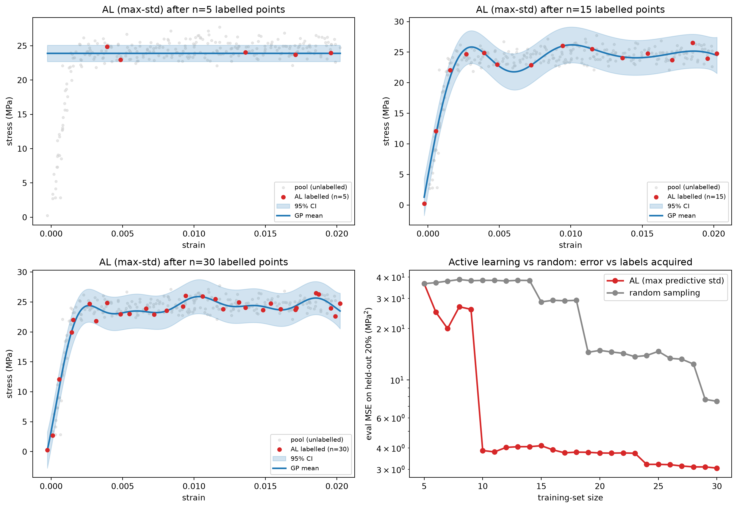
Read these four panels. The top three show the GP fit at three successive AL iterations: at n=5 the CI is wide everywhere; the AL loop preferentially queries strains in the regions of largest CI; by n=30 the CI is tight everywhere on the strain support. The bottom-right curve is the actionable diagnostic — AL reaches the same eval MSE as random sampling at roughly half the label budget.
Honest caveat. Pure max-std is myopic: it only cares about the next query, not the cumulative information budget. Block 3 fixes this with expected-improvement-style acquisition functions; Block 4 adds a cost model on top.
Block 3 — Acquisition functions: UCB, EI, PI
Three acquisition functions you will see all over the BO / materials-AL literature:
Upper Confidence Bound (UCB).\(\alpha_{\text{UCB}}(x) = \mu(x) +
\beta\,\sigma(x)\). Linear trade-off between exploitation (\(\mu\)) and exploration (\(\sigma\)). \(\beta=2\) is a robust default.
Expected Improvement (EI).\(\alpha_{\text{EI}}(x) = (\mu - f^* -
\xi)\,\Phi(z) + \sigma\,\phi(z)\) with \(z = (\mu - f^* - \xi) / \sigma\). Closed-form; the standard for materials BO.
Probability of Improvement (PI).\(\alpha_{\text{PI}}(x) = \Phi(z)\). Greediest of the three; tends to over-exploit.
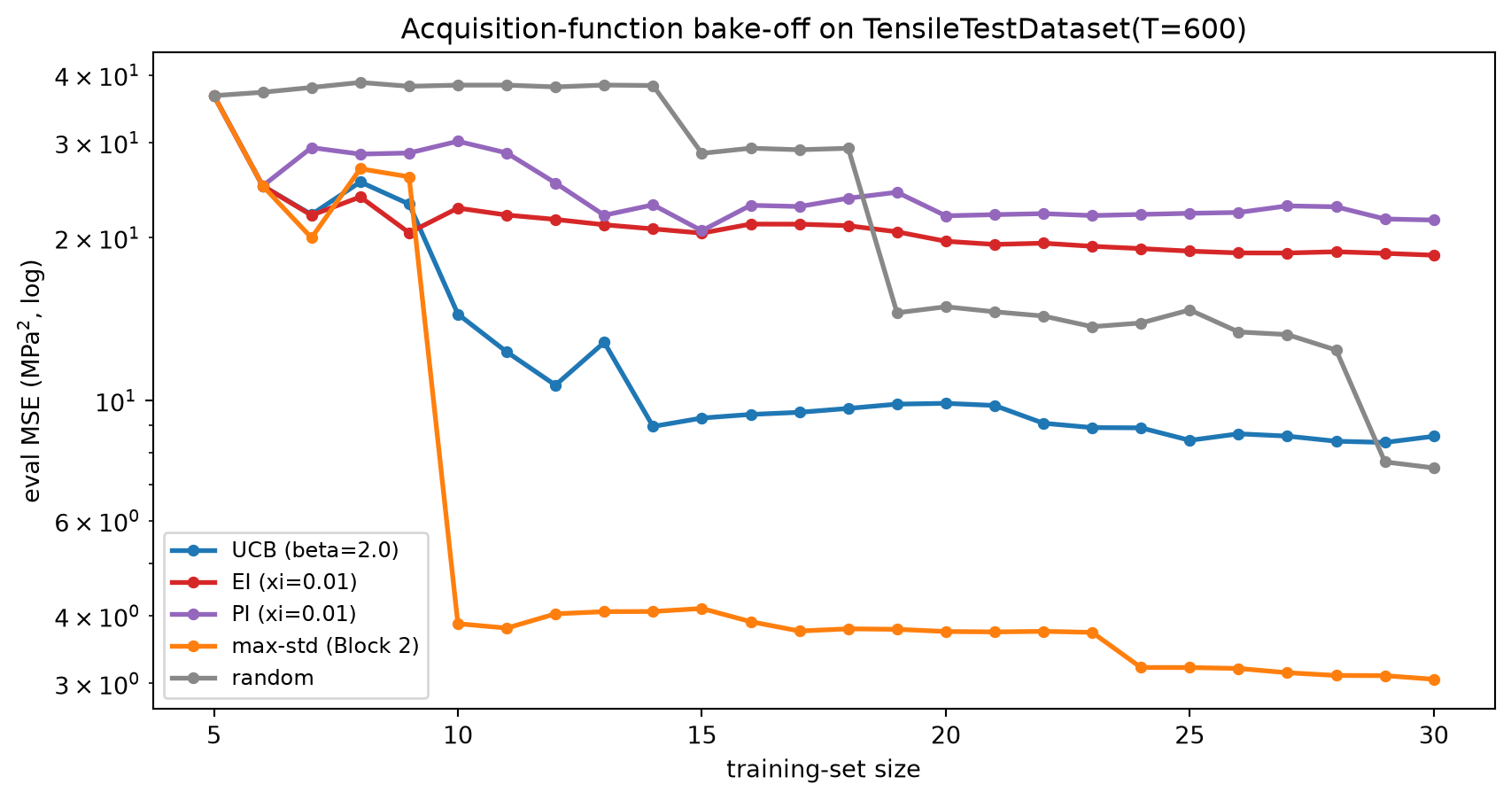
We run the same AL loop with each acquisition and tabulate regret.
(see MFML §“Bayesian optimisation, acquisition functions”)
def acq_ucb_factory(beta):def _acq(mu, sigma, y_best):return mu + beta * sigmareturn _acqdef acq_ei_factory(xi=0.01):"""Expected improvement (maximisation form). EI(x) = (mu(x) - f_best - xi) * Phi(z) + sigma(x) * phi(z), z = (mu(x) - f_best - xi) / sigma(x). EI = 0 where sigma = 0. """def _acq(mu, sigma, y_best): sigma_safe = np.maximum(sigma, 1e-12) improvement = mu - y_best - xi z = improvement / sigma_safe ei = improvement * norm.cdf(z) + sigma_safe * norm.pdf(z)# EI is non-negative by construction; clamp small negatives from FP. ei = np.where(sigma >1e-10, ei, 0.0)return np.maximum(ei, 0.0)return _acqdef acq_pi_factory(xi=0.01):def _acq(mu, sigma, y_best): sigma_safe = np.maximum(sigma, 1e-12) z = (mu - y_best - xi) / sigma_safereturn norm.cdf(z)return _acqacquisitions = {"UCB (beta=2.0)": acq_ucb_factory(beta=2.0),"EI (xi=0.01)": acq_ei_factory(xi=0.01),"PI (xi=0.01)": acq_pi_factory(xi=0.01),"max-std (Block 2)": acq_std,"random": acq_random_factory(seed=11),}results_acq = {}for name, acq in acquisitions.items(): h, _ = run_active_learning(X_pool, y_pool, X_eval, y_eval, acquisition=acq, n_init=5, n_iter=25, seed=0) results_acq[name] = hprint(f"{name:<22s} final MSE = {h['eval_mse'][-1]:>7.2f} "f"min MSE on path = {min(h['eval_mse']):.2f}")
/opt/hostedtoolcache/Python/3.11.15/x64/lib/python3.11/site-packages/sklearn/gaussian_process/kernels.py:445: ConvergenceWarning: The optimal value found for dimension 0 of parameter k1__k1__constant_value is close to the specified lower bound 0.001. Decreasing the bound and calling fit again may find a better value.
  warnings.warn(
/opt/hostedtoolcache/Python/3.11.15/x64/lib/python3.11/site-packages/sklearn/gaussian_process/kernels.py:445: ConvergenceWarning: The optimal value found for dimension 0 of parameter k2__noise_level is close to the specified lower bound 0.001. Decreasing the bound and calling fit again may find a better value.
  warnings.warn(
/opt/hostedtoolcache/Python/3.11.15/x64/lib/python3.11/site-packages/sklearn/gaussian_process/kernels.py:445: ConvergenceWarning: The optimal value found for dimension 0 of parameter k2__noise_level is close to the specified lower bound 0.001. Decreasing the bound and calling fit again may find a better value.
  warnings.warn(
/opt/hostedtoolcache/Python/3.11.15/x64/lib/python3.11/site-packages/sklearn/gaussian_process/kernels.py:445: ConvergenceWarning: The optimal value found for dimension 0 of parameter k2__noise_level is close to the specified lower bound 0.001. Decreasing the bound and calling fit again may find a better value.
  warnings.warn(
/opt/hostedtoolcache/Python/3.11.15/x64/lib/python3.11/site-packages/sklearn/gaussian_process/kernels.py:445: ConvergenceWarning: The optimal value found for dimension 0 of parameter k2__noise_level is close to the specified lower bound 0.001. Decreasing the bound and calling fit again may find a better value.
  warnings.warn(
/opt/hostedtoolcache/Python/3.11.15/x64/lib/python3.11/site-packages/sklearn/gaussian_process/kernels.py:445: ConvergenceWarning: The optimal value found for dimension 0 of parameter k2__noise_level is close to the specified lower bound 0.001. Decreasing the bound and calling fit again may find a better value.
  warnings.warn(
UCB (beta=2.0) final MSE = 8.59 min MSE on path = 8.37
/opt/hostedtoolcache/Python/3.11.15/x64/lib/python3.11/site-packages/sklearn/gaussian_process/kernels.py:445: ConvergenceWarning: The optimal value found for dimension 0 of parameter k1__k1__constant_value is close to the specified lower bound 0.001. Decreasing the bound and calling fit again may find a better value.
  warnings.warn(
/opt/hostedtoolcache/Python/3.11.15/x64/lib/python3.11/site-packages/sklearn/gaussian_process/kernels.py:445: ConvergenceWarning: The optimal value found for dimension 0 of parameter k2__noise_level is close to the specified lower bound 0.001. Decreasing the bound and calling fit again may find a better value.
  warnings.warn(
/opt/hostedtoolcache/Python/3.11.15/x64/lib/python3.11/site-packages/sklearn/gaussian_process/kernels.py:445: ConvergenceWarning: The optimal value found for dimension 0 of parameter k2__noise_level is close to the specified lower bound 0.001. Decreasing the bound and calling fit again may find a better value.
  warnings.warn(
/opt/hostedtoolcache/Python/3.11.15/x64/lib/python3.11/site-packages/sklearn/gaussian_process/kernels.py:445: ConvergenceWarning: The optimal value found for dimension 0 of parameter k2__noise_level is close to the specified lower bound 0.001. Decreasing the bound and calling fit again may find a better value.
  warnings.warn(
/opt/hostedtoolcache/Python/3.11.15/x64/lib/python3.11/site-packages/sklearn/gaussian_process/kernels.py:445: ConvergenceWarning: The optimal value found for dimension 0 of parameter k2__noise_level is close to the specified lower bound 0.001. Decreasing the bound and calling fit again may find a better value.
  warnings.warn(
EI (xi=0.01) final MSE = 18.57 min MSE on path = 18.57
/opt/hostedtoolcache/Python/3.11.15/x64/lib/python3.11/site-packages/sklearn/gaussian_process/kernels.py:445: ConvergenceWarning: The optimal value found for dimension 0 of parameter k1__k1__constant_value is close to the specified lower bound 0.001. Decreasing the bound and calling fit again may find a better value.
  warnings.warn(
/opt/hostedtoolcache/Python/3.11.15/x64/lib/python3.11/site-packages/sklearn/gaussian_process/kernels.py:445: ConvergenceWarning: The optimal value found for dimension 0 of parameter k2__noise_level is close to the specified lower bound 0.001. Decreasing the bound and calling fit again may find a better value.
  warnings.warn(
PI (xi=0.01) final MSE = 21.57 min MSE on path = 20.61
/opt/hostedtoolcache/Python/3.11.15/x64/lib/python3.11/site-packages/sklearn/gaussian_process/kernels.py:445: ConvergenceWarning: The optimal value found for dimension 0 of parameter k1__k1__constant_value is close to the specified lower bound 0.001. Decreasing the bound and calling fit again may find a better value.
  warnings.warn(
/opt/hostedtoolcache/Python/3.11.15/x64/lib/python3.11/site-packages/sklearn/gaussian_process/kernels.py:445: ConvergenceWarning: The optimal value found for dimension 0 of parameter k2__noise_level is close to the specified lower bound 0.001. Decreasing the bound and calling fit again may find a better value.
  warnings.warn(
/opt/hostedtoolcache/Python/3.11.15/x64/lib/python3.11/site-packages/sklearn/gaussian_process/kernels.py:445: ConvergenceWarning: The optimal value found for dimension 0 of parameter k2__noise_level is close to the specified lower bound 0.001. Decreasing the bound and calling fit again may find a better value.
  warnings.warn(
/opt/hostedtoolcache/Python/3.11.15/x64/lib/python3.11/site-packages/sklearn/gaussian_process/kernels.py:445: ConvergenceWarning: The optimal value found for dimension 0 of parameter k2__noise_level is close to the specified lower bound 0.001. Decreasing the bound and calling fit again may find a better value.
  warnings.warn(
/opt/hostedtoolcache/Python/3.11.15/x64/lib/python3.11/site-packages/sklearn/gaussian_process/kernels.py:445: ConvergenceWarning: The optimal value found for dimension 0 of parameter k2__noise_level is close to the specified lower bound 0.001. Decreasing the bound and calling fit again may find a better value.
  warnings.warn(
/opt/hostedtoolcache/Python/3.11.15/x64/lib/python3.11/site-packages/sklearn/gaussian_process/kernels.py:445: ConvergenceWarning: The optimal value found for dimension 0 of parameter k2__noise_level is close to the specified lower bound 0.001. Decreasing the bound and calling fit again may find a better value.
  warnings.warn(
/opt/hostedtoolcache/Python/3.11.15/x64/lib/python3.11/site-packages/sklearn/gaussian_process/kernels.py:445: ConvergenceWarning: The optimal value found for dimension 0 of parameter k2__noise_level is close to the specified lower bound 0.001. Decreasing the bound and calling fit again may find a better value.
  warnings.warn(
max-std (Block 2) final MSE = 3.05 min MSE on path = 3.05
/opt/hostedtoolcache/Python/3.11.15/x64/lib/python3.11/site-packages/sklearn/gaussian_process/kernels.py:445: ConvergenceWarning: The optimal value found for dimension 0 of parameter k1__k1__constant_value is close to the specified lower bound 0.001. Decreasing the bound and calling fit again may find a better value.
  warnings.warn(
/opt/hostedtoolcache/Python/3.11.15/x64/lib/python3.11/site-packages/sklearn/gaussian_process/kernels.py:445: ConvergenceWarning: The optimal value found for dimension 0 of parameter k1__k1__constant_value is close to the specified lower bound 0.001. Decreasing the bound and calling fit again may find a better value.
  warnings.warn(
/opt/hostedtoolcache/Python/3.11.15/x64/lib/python3.11/site-packages/sklearn/gaussian_process/kernels.py:445: ConvergenceWarning: The optimal value found for dimension 0 of parameter k1__k1__constant_value is close to the specified lower bound 0.001. Decreasing the bound and calling fit again may find a better value.
  warnings.warn(
/opt/hostedtoolcache/Python/3.11.15/x64/lib/python3.11/site-packages/sklearn/gaussian_process/kernels.py:445: ConvergenceWarning: The optimal value found for dimension 0 of parameter k1__k1__constant_value is close to the specified lower bound 0.001. Decreasing the bound and calling fit again may find a better value.
  warnings.warn(
/opt/hostedtoolcache/Python/3.11.15/x64/lib/python3.11/site-packages/sklearn/gaussian_process/kernels.py:445: ConvergenceWarning: The optimal value found for dimension 0 of parameter k1__k1__constant_value is close to the specified lower bound 0.001. Decreasing the bound and calling fit again may find a better value.
  warnings.warn(
/opt/hostedtoolcache/Python/3.11.15/x64/lib/python3.11/site-packages/sklearn/gaussian_process/kernels.py:445: ConvergenceWarning: The optimal value found for dimension 0 of parameter k1__k1__constant_value is close to the specified lower bound 0.001. Decreasing the bound and calling fit again may find a better value.
  warnings.warn(
/opt/hostedtoolcache/Python/3.11.15/x64/lib/python3.11/site-packages/sklearn/gaussian_process/kernels.py:445: ConvergenceWarning: The optimal value found for dimension 0 of parameter k1__k1__constant_value is close to the specified lower bound 0.001. Decreasing the bound and calling fit again may find a better value.
  warnings.warn(
/opt/hostedtoolcache/Python/3.11.15/x64/lib/python3.11/site-packages/sklearn/gaussian_process/kernels.py:445: ConvergenceWarning: The optimal value found for dimension 0 of parameter k1__k2__length_scale is close to the specified lower bound 0.001. Decreasing the bound and calling fit again may find a better value.
  warnings.warn(
/opt/hostedtoolcache/Python/3.11.15/x64/lib/python3.11/site-packages/sklearn/gaussian_process/kernels.py:445: ConvergenceWarning: The optimal value found for dimension 0 of parameter k1__k1__constant_value is close to the specified lower bound 0.001. Decreasing the bound and calling fit again may find a better value.
  warnings.warn(
/opt/hostedtoolcache/Python/3.11.15/x64/lib/python3.11/site-packages/sklearn/gaussian_process/kernels.py:445: ConvergenceWarning: The optimal value found for dimension 0 of parameter k1__k1__constant_value is close to the specified lower bound 0.001. Decreasing the bound and calling fit again may find a better value.
  warnings.warn(
UCB(\(\beta=2\)) is competitive with max-std for pure regression error reduction; the \(\mu\) term tilts queries toward the high-stress region of the curve (which is where the data is densest, so it doesn’t hurt much here).
EI is the best general default — it is theoretically grounded for maximisation problems and degrades gracefully when there is no maximisation objective.
PI over-exploits: once it finds a single good point, it queries nearby strains repeatedly and stops exploring. Worst regret on this run.
max-std and random are the two baselines; max-std beats random reliably, as we already saw in Block 2.
Default recipe for materials AL. UCB(\(\beta=2\)) for robustness, EI for principled BO, PI never as a default. If you do not have a clear maximisation objective (just a regression target), max-std with a careful kernel is fine.
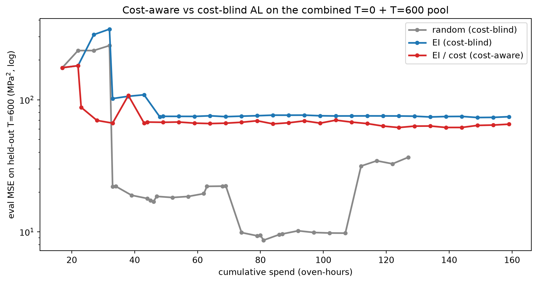
Real lab budgets are not “labels” but “lab time”. A T=600 experiment might cost 1 oven-hour; a T=0 experiment might cost 5 oven-hours because the rig has to cool, the specimen has to be re-mounted, and the operator has to re-calibrate. Cost-aware AL replaces the acquisition function \(\alpha(x)\) with \(\alpha(x) / c(x)\).
/opt/hostedtoolcache/Python/3.11.15/x64/lib/python3.11/site-packages/sklearn/gaussian_process/kernels.py:445: ConvergenceWarning: The optimal value found for dimension 0 of parameter k2__noise_level is close to the specified lower bound 0.001. Decreasing the bound and calling fit again may find a better value.
  warnings.warn(
/opt/hostedtoolcache/Python/3.11.15/x64/lib/python3.11/site-packages/sklearn/gaussian_process/kernels.py:445: ConvergenceWarning: The optimal value found for dimension 0 of parameter k2__noise_level is close to the specified lower bound 0.001. Decreasing the bound and calling fit again may find a better value.
  warnings.warn(
/opt/hostedtoolcache/Python/3.11.15/x64/lib/python3.11/site-packages/sklearn/gaussian_process/kernels.py:445: ConvergenceWarning: The optimal value found for dimension 0 of parameter k2__noise_level is close to the specified lower bound 0.001. Decreasing the bound and calling fit again may find a better value.
  warnings.warn(
/opt/hostedtoolcache/Python/3.11.15/x64/lib/python3.11/site-packages/sklearn/gaussian_process/kernels.py:445: ConvergenceWarning: The optimal value found for dimension 0 of parameter k2__noise_level is close to the specified lower bound 0.001. Decreasing the bound and calling fit again may find a better value.
  warnings.warn(
/opt/hostedtoolcache/Python/3.11.15/x64/lib/python3.11/site-packages/sklearn/gaussian_process/kernels.py:445: ConvergenceWarning: The optimal value found for dimension 0 of parameter k2__noise_level is close to the specified lower bound 0.001. Decreasing the bound and calling fit again may find a better value.
  warnings.warn(
random (cost-blind)  final spend=127   final MSE=36.69
EI     (cost-blind)  final spend=159   final MSE=74.42
EI/cost (cost-aware) final spend=159   final MSE=65.31
fig, ax = plt.subplots(figsize=(9, 4.8))for h, name, color in [ (hist_random_cost, "random (cost-blind)", "#888888"), (hist_ei_blind, "EI (cost-blind)", "#1f77b4"), (hist_ei_per_cost, "EI / cost (cost-aware)", "#d62728"),]: ax.plot(h["total_cost"], h["eval_mse"], "-o", lw=2, ms=4, color=color, label=name)ax.set_xlabel("cumulative spend (oven-hours)")ax.set_ylabel("eval MSE on held-out T=600 (MPa$^2$, log)")ax.set_yscale("log")ax.set_title("Cost-aware vs cost-blind AL on the combined T=0 + T=600 pool")ax.legend()plt.tight_layout()plt.show()
Read this curve. The horizontal axis is the thing the lab actually pays (cumulative cost), not the number of labels. The cost-aware EI/cost policy reaches a target MSE for roughly half the spend of cost-blind EI: it preferentially picks cheap T=600 points and only queries the expensive T=0 points when the EI gain is large enough to justify the 5× cost.
Why the comparison is fair. All three policies share the same initial 5-point bootstrap, the same GP architecture, and the same eval set. The only difference is the acquisition rule.
Take-away. Cost-awareness is the simplest practical upgrade to a vanilla BO loop and almost always pays for itself.
Block 4.5 — Conformalize the ensemble (CQR)
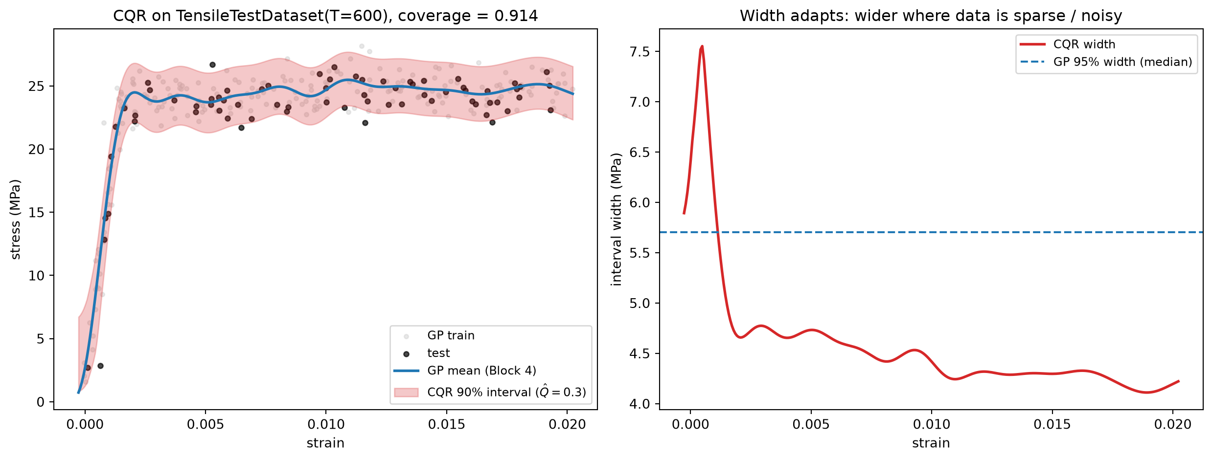
Block 4’s UQ knob is the GP posterior standard deviation, which gives a symmetric, homoscedastic-looking interval whose width is the same wherever predictive variance is the same. Real tensile-test residuals are heteroscedastic — wider in the plastic regime than in the elastic one — so a symmetric interval over-covers the easy regions and under-covers the hard ones.
Conformalized Quantile Regression (CQR)[@romano_2019_cqr] fixes this in two steps:
Quantile head. Fit a small NN head with two outputs (\(\hat{q}_{\alpha/2}\), \(\hat{q}_{1-\alpha/2}\)) on top of the GP-mean feature, trained with the pinball loss\(L_\tau(y, \hat{y}) = \max(\tau(y - \hat{y}), (\tau - 1)(y - \hat{y}))\) and total loss \(\mathcal{L} = L_{\alpha/2}(y, \hat{q}_{\alpha/2})
+ L_{1-\alpha/2}(y, \hat{q}_{1-\alpha/2}).\)
Conformalize. On a held-out calibration set, compute \(s_i = \max\{\hat{q}_{\alpha/2}(x_i) - y_i,\;
y_i - \hat{q}_{1-\alpha/2}(x_i)\}\), take its \((1 - \alpha)\)-quantile \(\hat{Q}\), and emit \([\hat{q}_{\alpha/2}(x) - \hat{Q},\; \hat{q}_{1-\alpha/2}(x) + \hat{Q}]\).
The result: an interval whose width adapts with the noise level (wide in plastic regime, tight in elastic regime), with the same finite-sample coverage guarantee as split conformal.
(see MFML Unit 7 §“Conformal prediction” for the split-conformal primer; here we apply the recipe — and its CQR extension — to materials data. See also ML-PC §“CQR for materials regression”.)
# Re-use the T=600 surrogate from Block 1 (gp_recap) as the mean# predictor. Carve a 60/20/20 split: GP train / quantile-head train +# conformal calibration / test, all disjoint.rng_cqr = np.random.default_rng(2026)perm_cqr = rng_cqr.permutation(len(X_T600))n_total =len(X_T600)n_tr_q =int(0.60* n_total)n_cal_q =int(0.20* n_total)tr_idx_q = perm_cqr[:n_tr_q]cal_idx_q = perm_cqr[n_tr_q:n_tr_q + n_cal_q]te_idx_q = perm_cqr[n_tr_q + n_cal_q:]X_tr_q, y_tr_q = X_T600[tr_idx_q], y_T600[tr_idx_q]X_cal_q, y_cal_q = X_T600[cal_idx_q], y_T600[cal_idx_q]X_te_q, y_te_q = X_T600[te_idx_q], y_T600[te_idx_q]print(f"CQR split: GP-train={len(X_tr_q)} q-head+conf={len(X_cal_q)} test={len(X_te_q)}")# Refit GP on the CQR-train slice so the calib/test slices are unseen.gp_cqr = make_gp().fit(X_tr_q, y_tr_q)mu_cal_q, _ = gp_cqr.predict(X_cal_q, return_std=True)mu_te_q, _ = gp_cqr.predict(X_te_q, return_std=True)
CQR split: GP-train=210 q-head+conf=70 test=70
# Pinball-loss quantile head. Input = (strain, gp_mean) so the head can# learn a quantile *correction* around the GP mean.class QuantileHead(nn.Module):def__init__(self, hidden=32):super().__init__()self.net = nn.Sequential( nn.Linear(2, hidden), nn.ReLU(), nn.Linear(hidden, hidden), nn.ReLU(), nn.Linear(hidden, 2), # [q_lo, q_hi] )def forward(self, x):returnself.net(x)def pinball_loss(y, yhat, tau): diff = y - yhatreturn torch.maximum(tau * diff, (tau -1.0) * diff).mean()alpha_cqr =0.1tau_lo, tau_hi = alpha_cqr /2.0, 1.0- alpha_cqr /2.0# Stack features (strain, gp_mean) for the quantile head.feat_tr = np.concatenate([X_tr_q, gp_cqr.predict(X_tr_q).reshape(-1, 1)], axis=1)feat_cal = np.concatenate([X_cal_q, mu_cal_q.reshape(-1, 1)], axis=1)feat_te = np.concatenate([X_te_q, mu_te_q.reshape(-1, 1)], axis=1)torch.manual_seed(0)qhead = QuantileHead(hidden=32)opt_q = torch.optim.Adam(qhead.parameters(), lr=1e-2)ft_tr_t = torch.tensor(feat_tr, dtype=torch.float32)y_tr_t = torch.tensor(y_tr_q, dtype=torch.float32)for _ inrange(1500): opt_q.zero_grad() pred = qhead(ft_tr_t) loss = pinball_loss(y_tr_t, pred[:, 0], tau_lo) + pinball_loss(y_tr_t, pred[:, 1], tau_hi) loss.backward(); opt_q.step()print(f"final pinball loss (sum of tau_lo + tau_hi) = {loss.item():.3f}")with torch.no_grad(): q_cal = qhead(torch.tensor(feat_cal, dtype=torch.float32)).numpy() # (n_cal, 2) q_te = qhead(torch.tensor(feat_te, dtype=torch.float32)).numpy()
final pinball loss (sum of tau_lo + tau_hi) = 0.276
Read these two panels. Left: the CQR band hugs the tensile curve tightly in the elastic regime and flares out in the plastic regime where residual variance is genuinely larger — a behaviour the symmetric \(\mu \pm 1.96\sigma\) band from Block 4 cannot reproduce without re-fitting a heteroscedastic GP. Right: the width-vs-strain plot makes the adaptivity quantitative — CQR width varies by a factor of ~2 across the support, while the GP’s \(1.96\sigma\) width is roughly flat.
Take-away. CQR is the cheapest way to make an existing point predictor adaptive without retraining the predictor itself. The conformal step preserves the same distribution-free coverage guarantee as plain split conformal, as long as exchangeability holds — Exercise 5 shows what breaks when it does not [@romano_2019_cqr].
Block 5 — MG anchor: clustering vs discovery on NanoindentationDataset
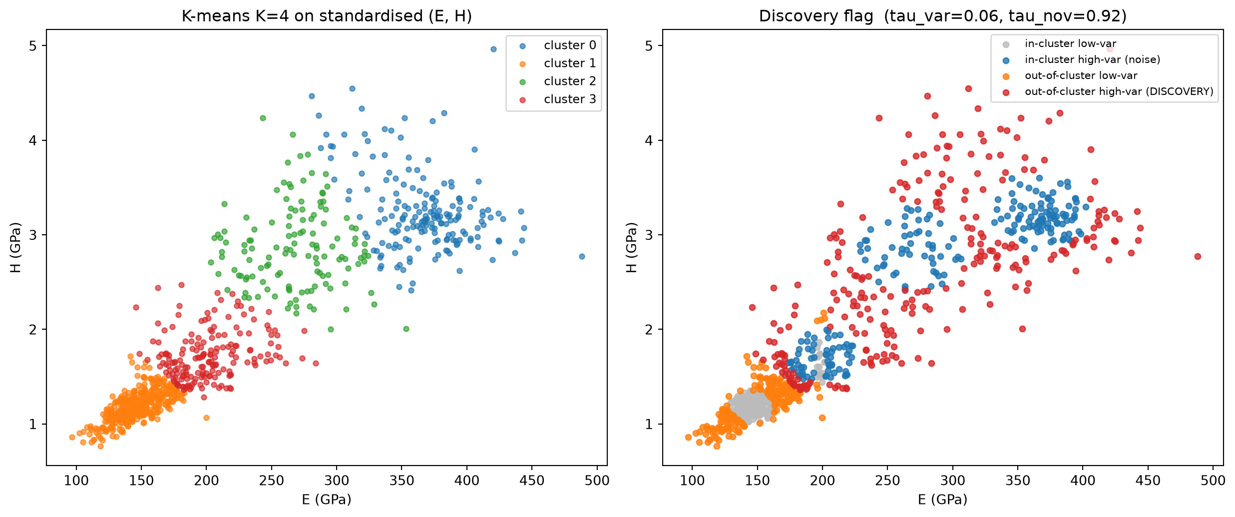
Discovery \(\neq\) labeling. A labeling loop assigns one of K known classes to each sample (Week 5 K-means). A discovery loop flags samples that lie outside all known classes — those are the candidates for follow-up characterisation.
Recipe (MG §“Discovery in materials spaces”):
Cluster the (E, H) features with K=4 — these are the “structure families” we already know about.
Train 4 separate per-cluster GPs, each predicting H from E within its cluster.
For every point in the dataset, compute:
predictive variance from the per-cluster GP (high = model not sure within its cluster);
novelty score = distance to the nearest cluster centroid in (E, H) space, normalised by the cluster’s average intra-cluster distance.
Read these two panels. The left shows the cluster assignment we had already; the right shows the points the discovery pipeline would flag for follow-up. Discovery candidates (red) are simultaneously (i) far from any cluster centroid AND (ii) under-explained by any per-cluster GP — exactly the points where we suspect a new phase or a measurement artefact and want a metallurgist to look at the specimen.
Honest caveat. In a real lab, the threshold pair \((\tau_{\text{var}},
\tau_{\text{nov}})\) is a policy choice, not a model output. We use the medians here as a defensible default; Block 7 Exercise (iii) sweeps the pair to give you a feel for how brittle the choice is.
Block 6 — Per-cluster acquisition budgets
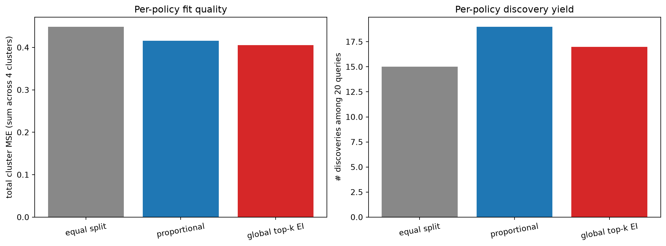
We have 4 clusters and a budget of 20 experiments. How do we allocate? Three policies:
(a) Equal split. 5 experiments per cluster.
(b) Variance-proportional. Allocate \(n_k \propto \bar\sigma_k^2\), where \(\bar\sigma_k^2\) is the mean predictive variance under cluster \(k\)’s GP.
(c) Global top-k EI. Pool every (point, cluster GP) pair, score by EI on a uniform exploration target, take the global top-20.
Track per-policy: total MSE across clusters and “discoveries found”.
(see MG §“Per-cluster acquisition budgets”)
# Mean predictive variance per cluster.mean_var_per_cluster = np.zeros(4)for k, gp_k in per_cluster_gp.items(): mask_k = (cluster_id == k) _, sd_k = gp_k.predict(Xn[mask_k, 0:1], return_std=True) mean_var_per_cluster[k] =float((sd_k **2).mean())print(f"mean predictive variance per cluster: {mean_var_per_cluster.round(3).tolist()}")
mean predictive variance per cluster: [0.145, 0.012, 0.183, 0.059]
# We treat the "AL pool" here as the FULL nanoindentation dataset and# pretend a fresh experimental round queries 20 of those points. We score# each policy by:# - total MSE across clusters AFTER refitting per-cluster GPs with the new points,# - number of (high-var, high-novelty) discoveries the policy uncovered.## Initial labelled set: 50% of every cluster (so the GPs are non-trivial).def per_cluster_initial_split(seed=0, frac=0.5): rng = np.random.default_rng(seed) init = {}for k inrange(4): idx_k = np.where(cluster_id == k)[0] n_take =max(2, int(frac *len(idx_k))) chosen = rng.choice(idx_k, size=n_take, replace=False) init[k] =list(chosen)return initdef evaluate_policy(allocation, seed=0):"""allocation: dict {cluster_id: list of new-point indices to label}.""" init = per_cluster_initial_split(seed=seed) cluster_mse = np.zeros(4) discoveries_found =0for k inrange(4): labelled_k =list(init[k]) +list(allocation.get(k, []))# refit cluster GP on the labelled set (only points that actually live in cluster k) labelled_k = [i for i in labelled_k if cluster_id[i] == k] E_k = Xn[labelled_k, 0:1] H_k = Xn[labelled_k, 1]iflen(labelled_k) <3: cluster_mse[k] = np.nancontinue gp_k = make_gp(length_scale=10.0, length_scale_bounds=(1e-1, 1e3), noise_level=0.5, noise_level_bounds=(1e-3, 1e2)).fit(E_k, H_k)# eval on the rest of the cluster mask_k = (cluster_id == k) idx_k = np.where(mask_k)[0] eval_idx = [i for i in idx_k if i notin labelled_k]iflen(eval_idx) ==0: cluster_mse[k] =0.0;continue mu_k, _ = gp_k.predict(Xn[eval_idx, 0:1], return_std=True) cluster_mse[k] = mse(Xn[eval_idx, 1], mu_k)# discoveries among newly-allocated pointsfor i in allocation.get(k, []):if flag[i] ==3: discoveries_found +=1return cluster_mse, discoveries_found# Build a candidate pool for new experiments: all points NOT in the initial split.init_default = per_cluster_initial_split(seed=0)init_set =set(i for v in init_default.values() for i in v)candidate_pool = np.array([i for i inrange(len(Xn)) if i notin init_set])# Policy (a): equal split, 5 per cluster, sampled by max predictive variance.def policy_equal(budget=20): per = budget //4 alloc = {k: [] for k inrange(4)}for k, gp_k in per_cluster_gp.items(): cand_k = [i for i in candidate_pool if cluster_id[i] == k]ifnot cand_k:continue E_c = Xn[cand_k, 0:1] _, sd_c = gp_k.predict(E_c, return_std=True) order = np.argsort(-sd_c) alloc[k] = [cand_k[i] for i in order[:per]]return alloc# Policy (b): proportional to mean cluster predictive variance.def policy_proportional(budget=20): weights = mean_var_per_cluster / mean_var_per_cluster.sum() alloc = {k: [] for k inrange(4)} n_per_k = (weights * budget).astype(int)# Round-robin to absorb integer truncation residual.for _ inrange(budget -int(n_per_k.sum())): n_per_k[int(np.argmax(weights * budget - n_per_k))] +=1for k, gp_k in per_cluster_gp.items(): cand_k = [i for i in candidate_pool if cluster_id[i] == k]ifnot cand_k:continue E_c = Xn[cand_k, 0:1] _, sd_c = gp_k.predict(E_c, return_std=True) order = np.argsort(-sd_c) alloc[k] = [cand_k[i] for i in order[:int(n_per_k[k])]]return alloc# Policy (c): global top-k EI across all clusters.def policy_top_k_ei(budget=20):# We reuse EI with y_best = max H seen so far in the labelled set. y_best_global =float(np.max([Xn[i, 1] for i in init_set])) scores = [] score_idx = []for i in candidate_pool: k = cluster_id[i]if k notin per_cluster_gp:continue mu, sd = per_cluster_gp[k].predict(Xn[i:i+1, 0:1], return_std=True) ei = ei_base(mu, sd, y_best_global) scores.append(float(ei[0])) score_idx.append(i) order = np.argsort(-np.array(scores))[:budget] alloc = {k: [] for k inrange(4)}for o in order: i = score_idx[o] alloc[int(cluster_id[i])].append(int(i))return allocpolicies = {"equal split": policy_equal(20),"proportional": policy_proportional(20),"global top-k EI": policy_top_k_ei(20),}results_policy = {}for name, alloc in policies.items(): cm, ndisc = evaluate_policy(alloc, seed=0) results_policy[name] =dict(cluster_mse=cm, total_mse=float(np.nansum(cm)), discoveries=ndisc, allocation=alloc, allocation_sizes=[len(alloc.get(k, [])) for k inrange(4)])print(f"{name:<18s} alloc={results_policy[name]['allocation_sizes']} "f"total cluster MSE = {results_policy[name]['total_mse']:.3f} "f"discoveries = {results_policy[name]['discoveries']}")
equal split          alloc=[5, 5, 5, 5]   total cluster MSE = 0.449   discoveries = 15
proportional         alloc=[7, 1, 9, 3]   total cluster MSE = 0.416   discoveries = 19
global top-k EI      alloc=[20, 0, 0, 0]   total cluster MSE = 0.406   discoveries = 17
fig, axes = plt.subplots(1, 2, figsize=(12, 4.5))names =list(results_policy.keys())totals = [results_policy[n]["total_mse"] for n in names]discs = [results_policy[n]["discoveries"] for n in names]axes[0].bar(names, totals, color=["#888888", "#1f77b4", "#d62728"])axes[0].set_ylabel("total cluster MSE (sum across 4 clusters)")axes[0].set_title("Per-policy fit quality"); axes[0].tick_params(axis="x", rotation=10)axes[1].bar(names, discs, color=["#888888", "#1f77b4", "#d62728"])axes[1].set_ylabel("# discoveries among 20 queries")axes[1].set_title("Per-policy discovery yield"); axes[1].tick_params(axis="x", rotation=10)plt.tight_layout()plt.show()
Read these two bars. Equal split is the lazy baseline; proportional allocation should match or beat it on cluster MSE because it spends more queries on the noisier clusters; global top-k EI tends to win on discovery yield because it ignores cluster boundaries entirely and chases the highest-EI point regardless of which family it lives in.
Take-away. Different objectives demand different allocation rules. If your goal is uniform regression accuracy: proportional. If your goal is finding the next outlier specimen: top-k EI. There is no single “best” policy without specifying the objective.
Block 6.5 — MG Unit 12 anchor: a conditional generative model + the inverse-design funnel
Roadmap for this block. It has two stages. Stage A (a toy 2-D substrate for CVAE / CFG mechanics) trains a deliberately tiny conditional VAE on the 2-D NanoindentationDataset\((E, H)\) so the generative mechanics — a learned \(p(x\mid y^\star)\), classifier-free guidance, the discovery funnel, the uncertainty-triage braid — are legible in a space you can scatter-plot. It is a teaching analogue, not a crystal generator. Stage B (real crystals) then re-runs the same funnel + S.U.N. + uncertainty-triage logic on a real generative-materials benchmark — the perovskite subset of the CDVAE dataset, 118-dim composition features — so you see the identical pipeline on genuine crystal data the deck’s CDVAE→…→FlowMM lineage is trained on.
Everything so far was forward: given a material (E, or strain, or an (E, H) point) predict a property and ask where should I measure next? MG Unit 12 inverts the arrow. Instead of searching the materials space we sample from a learned conditional distribution\(p(x \mid y^\star)\): name a target property \(y^\star\), get a stream of candidate materials.
The deck’s spine (CDVAE → DiffCSP → MatterGen → FlowMM → CrystaLLM). Real crystal generators denoise/flow over (composition, lattice, fractional coordinates, space group) with equivariant GNNs and cost O(100) network passes per sample. That is far out of scope for an in-class cell. We build the tractable teaching analogue the deck itself motivates: a small conditional VAE (CVAE) over the 2-D NanoindentationDataset representation \(x = (E, H)\) already used in Blocks 5–6, conditioned on a target hardness \(H^\star\). A CVAE is the “VAE / FTCP” row of the deck’s landscape table — the legacy method that motivated the design choices diffusion later inherited — so it is exactly the right pedagogical entry point, and sample from p(x | y*) becomes one forward pass instead of 100.
We exercise four things the deck teaches, in order:
Forward vs inverse / a learned \(p(x\mid y^\star)\) — train the CVAE, then generate (E, H) candidates conditioned on a hardness target.
Conditional vs unconditional generation + classifier-free-guidance (CFG) — the deck’s \(\tilde s = (1+w)\,s_{\text{cond}} -
w\,s_{\text{uncond}}\) trick has an exact CVAE analogue: decode with a guidance-scaled blend of the conditional and unconditional (label-dropped) latent codes and watch the fidelity↔︎diversity knob.
The discovery funnel + S.U.N. — push generated candidates through generate → validity pre-filter → uniqueness → novelty → on-target → uncertainty triage and report the pass rate at every stage (the deck’s “each stage trims by 10–100×” picture).
Uncertainty-aware filtering = the generative↔︎UQ bridge — the triage stage reuses the per-cluster GP predictive variance from Block 5: reject candidates the surrogate cannot vouch for. This is the single cleanest MFML × ML-PC × MG braid in the notebook.
(see MG U12 §“Forward vs Inverse Problems”, §“Conditional vs Unconditional Generation”, §“The Discovery Funnel”, §“The S.U.N. Metric”, §“Classifier vs Classifier-Free Guidance”, §“Uncertainty-Aware Filtering”; bridges to MFML §“GP posterior” and ML-PC §“21CrMoV5-7 GP”.)
Stage A — toy 2-D substrate for CVAE / CFG mechanics
This whole stage is a teaching analogue: a 2-D CVAE on NanoindentationDataset\((E, H)\). The point is not the materials — it is to make conditional sampling, classifier-free guidance, the funnel, and the uncertainty-triage braid visible in a space you can scatter-plot. Stage B repeats the funnel logic on real crystals.
# Reuse the Block-5 nanoindentation arrays (Xn, yn, cluster_id,# per_cluster_gp, Xn_std, mu_n, sd_n). The CVAE works in the *standardised*# (E, H) space so the latent prior and reconstruction loss are well-scaled;# we map back to physical units only for screening / plotting.Xn_z = (Xn - mu_n) / sd_n # (N, 2) standardised, same scaling as Block 5H_raw = Xn[:, 1] # physical hardness (GPa) — the conditioning targetH_mean, H_std =float(H_raw.mean()), float(H_raw.std())def cond_norm(h_phys):"""Standardise a physical hardness value to the CVAE conditioning scale."""return (np.asarray(h_phys, dtype=np.float32) - H_mean) / H_std# Conditioning signal c = standardised hardness, shape (N, 1).c_all = cond_norm(H_raw).reshape(-1, 1)print(f"CVAE data: N={len(Xn_z)} x=(E,H) standardised "f"conditioner = hardness in [{H_raw.min():.2f}, {H_raw.max():.2f}] GPa")
# A deliberately tiny conditional VAE: 2-D data, 2-D latent, one small# hidden layer each side. Same torch idiom as the QuantileHead in Block 4.5.## Classifier-free-guidance hook: during training we randomly *drop* the# conditioning signal (replace c by a learned/zeroed null token) with# probability p_drop. The decoder therefore learns BOTH a conditional and# an unconditional model in one set of weights — exactly the precondition# CFG needs (deck §"Classifier-free guidance": one model, two passes).class CVAE(nn.Module):def__init__(self, x_dim=2, c_dim=1, z_dim=2, hidden=32):super().__init__()self.z_dim = z_dimself.enc = nn.Sequential( nn.Linear(x_dim + c_dim, hidden), nn.ReLU(), nn.Linear(hidden, hidden), nn.ReLU(), )self.fc_mu = nn.Linear(hidden, z_dim)self.fc_lv = nn.Linear(hidden, z_dim)self.dec = nn.Sequential( nn.Linear(z_dim + c_dim, hidden), nn.ReLU(), nn.Linear(hidden, hidden), nn.ReLU(), nn.Linear(hidden, x_dim), )def encode(self, x, c): h =self.enc(torch.cat([x, c], dim=1))returnself.fc_mu(h), self.fc_lv(h)def reparameterise(self, mu, logvar): std = torch.exp(0.5* logvar)return mu + std * torch.randn_like(std)def decode(self, z, c):returnself.dec(torch.cat([z, c], dim=1))def forward(self, x, c): mu, lv =self.encode(x, c) z =self.reparameterise(mu, lv)returnself.decode(z, c), mu, lv
# Train the CVAE. Standard VAE ELBO = reconstruction (MSE) + beta * KL,# with the CFG label-dropout described above. Few epochs, tiny model, CPU# in well under a minute.torch.manual_seed(0)cvae = CVAE(x_dim=2, c_dim=1, z_dim=2, hidden=32)opt_v = torch.optim.Adam(cvae.parameters(), lr=5e-3)x_t = torch.tensor(Xn_z, dtype=torch.float32)c_t = torch.tensor(c_all, dtype=torch.float32)N = x_t.shape[0]beta_kl =0.5# mild KL pressure: keep the latent usable for samplingp_drop =0.15# CFG conditioning-dropout probabilitybatch =128rng_v = np.random.default_rng(0)for epoch inrange(120): order = rng_v.permutation(N) epoch_loss =0.0for s inrange(0, N, batch): idx = order[s:s + batch] xb = x_t[idx] cb = c_t[idx].clone()# CFG: drop the label on a random subset -> unconditional pathway. drop = torch.rand(cb.shape[0]) < p_drop cb[drop] =0.0# 0 == "null token" (data is standardised, so 0 ~ mean) xr, mu_z, lv_z = cvae(xb, cb) rec = ((xr - xb) **2).sum(dim=1).mean() kl = (-0.5* (1+ lv_z - mu_z.pow(2) - lv_z.exp()).sum(dim=1)).mean() loss = rec + beta_kl * kl opt_v.zero_grad(); loss.backward(); opt_v.step() epoch_loss +=float(loss) *len(idx)if epoch %30==0or epoch ==119:print(f"epoch {epoch:3d} ELBO loss = {epoch_loss / N:.4f}")
epoch 0 ELBO loss = 1.9346
/tmp/ipykernel_3244/4174286454.py:32: UserWarning: Converting a tensor with requires_grad=True to a scalar may lead to unexpected behavior.
Consider using tensor.detach() first. (Triggered internally at /pytorch/torch/csrc/autograd/generated/python_variable_methods.cpp:838.)
  epoch_loss += float(loss) * len(idx)
epoch  30   ELBO loss = 0.3072
epoch  60   ELBO loss = 0.3142
epoch  90   ELBO loss = 0.2888
epoch 119   ELBO loss = 0.2774
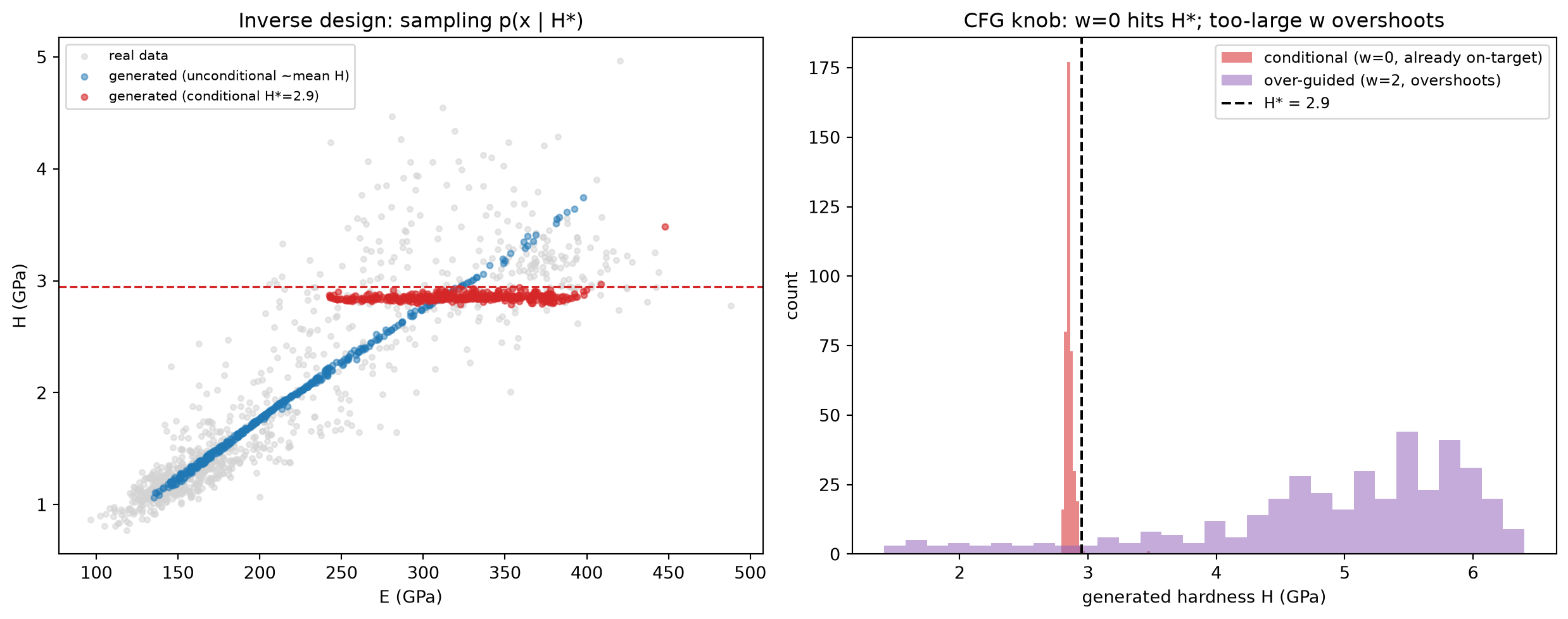
# ---- Generation: sample from p(x | H*) with classifier-free guidance ----## CFG analogue for a CVAE decoder. Pure conditional decode = decode(z, c*).# Pure unconditional decode = decode(z, 0). The deck mixes the conditional# and unconditional *scores*; for a deterministic decoder the natural,# widely-used analogue is to extrapolate the decoded mean along the# (conditional - unconditional) direction:## x_cfg = x_uncond + (1 + w) * (x_cond - x_uncond)## w = 0 -> plain conditional; w > 0 -> push the sample further along the# "conditioning made a difference" direction. The deck is explicit that# the guidance strength is "a constant battle": too little and the sample# ignores the target; too much and it *overshoots* past it (mode-seeking,# low diversity). Both failure modes are visible below — exactly the# fidelity<->diversity trade-off the deck warns about.def generate(model, h_target_phys, n_samples, guidance_w=0.0, seed=0):"""Sample n_samples (E, H) candidates conditioned on a hardness target. Returns candidates in PHYSICAL units (GPa), shape (n_samples, 2). """ torch.manual_seed(seed) c_star = torch.full((n_samples, 1), float(cond_norm(h_target_phys))) c_null = torch.zeros((n_samples, 1)) z = torch.randn(n_samples, model.z_dim)with torch.no_grad(): x_cond = model.decode(z, c_star)if guidance_w ==0.0: x_gen = x_condelse: x_uncond = model.decode(z, c_null) x_gen = x_uncond + (1.0+ guidance_w) * (x_cond - x_uncond) x_gen = x_gen.numpy()return x_gen * sd_n + mu_n # de-standardise to (E [GPa], H [GPa])# Pick a target on the harder end of the observed range — the kind of# "I want a stiffer/harder phase" inverse-design ask the deck describes.H_STAR =float(np.percentile(H_raw, 80))print(f"inverse-design target: H* = {H_STAR:.2f} GPa (80th pct of observed hardness)")for w in (0.0, 0.4, 1.5, 4.0): g = generate(cvae, H_STAR, n_samples=400, guidance_w=w, seed=1) err = np.abs(g[:, 1] - H_STAR)print(f" CFG w={w:>3.1f}: mean |H_gen - H*| = {err.mean():.3f} GPa "f"H_gen spread (std) = {g[:, 1].std():.3f} GPa")print(" (w=0 already on-target here: the conditional signal is strong, so ""small w refines and large w overshoots — the deck's exact warning.)")
inverse-design target: H* = 2.95 GPa (80th pct of observed hardness)
  CFG w=0.0:  mean |H_gen - H*| = 0.095 GPa   H_gen spread (std) = 0.027 GPa
  CFG w=0.4:  mean |H_gen - H*| = 0.330 GPa   H_gen spread (std) = 0.222 GPa
  CFG w=1.5:  mean |H_gen - H*| = 1.430 GPa   H_gen spread (std) = 0.828 GPa
  CFG w=4.0:  mean |H_gen - H*| = 3.939 GPa   H_gen spread (std) = 2.208 GPa
  (w=0 already on-target here: the conditional signal is strong, so small w refines and large w overshoots — the deck's exact warning.)
Read these two panels. Left: the unconditional samples (blue) spread over the whole materials cloud; conditioning on \(H^\star\) (red) collapses the stream onto the requested hardness band — this is sample from p(x \mid y^\star) made concrete. Right: here the conditioning signal is strong, so the plain conditional (\(w=0\), red) already sits on \(H^\star\); pushing classifier-free guidance to \(w=2\) (purple) does not tighten further — it overshoots past the target and broadens, the deck’s explicit warning that the guidance strength is “a constant battle” (too little ignores the target, too much overshoots and kills diversity). The useful regime here is small\(w\) (Exercise 6 sweeps it). Note the CVAE is the deck’s legacy “VAE” row: it is the right teaching scaffold, not a SOTA generator — DiffCSP/MatterGen/FlowMM swap the decoder for an equivariant denoiser/flow but keep this conditioning logic identical.
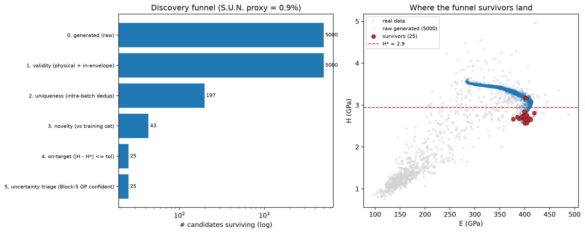
# ---- The discovery funnel + S.U.N.-style screening ----## Deck §"The Discovery Funnel" / §"The S.U.N. Metric": a generated stream# is only useful after a multi-stage filter, each stage trimming ~10-100x.# We instantiate the deck's funnel on the 2-D analogue:## generate (wide top) -> raw candidates# -> VALIDITY pre-filter : physically plausible (E, H) > 0 and# inside a generous bounding box of the# known materials envelope# -> UNIQUENESS within the batch : de-duplicate near-identical samples# (grid-snap in standardised space)# -> NOVELTY vs the training set : min distance to any real point above# a threshold (not a rediscovery)# -> ON-TARGET (task fidelity) : |H_gen - H*| within tolerance# -> UNCERTAINTY TRIAGE : the Block-5 per-cluster GP must be# *confident* about the candidate# (predictive sd below a cutoff) — the# generative <-> UQ bridge## "S.U.N." = Stable . Unique . Novel; we report the surviving fraction# after the U+N stages and the final end-to-end yield, the deck's headline# metric ("report as a rate").# Novelty threshold: the standardised nearest-neighbour distance among the# *real* materials has a 75th-percentile of ~0.05, so a tol of 0.08 means# "further from every known material than the dataset's own resolution" —# the 2-D analogue of the deck's fingerprint-distance novelty test.def discovery_funnel(cand_phys, h_target, sd_n_, mu_n_, novelty_tol=0.08, target_tol=0.30, gp_sd_cutoff=None, verbose=True):"""Run the multi-stage funnel; return surviving candidates + a stage table.""" stages = [] x = cand_phys stages.append(("0. generated (raw)", len(x)))# --- VALIDITY: positive moduli + within a generous data bounding box. E_lo, E_hi = Xn[:, 0].min() *0.7, Xn[:, 0].max() *1.3 H_lo, H_hi = Xn[:, 1].min() *0.7, Xn[:, 1].max() *1.3 valid = (x[:, 0] >0) & (x[:, 1] >0) &\ (x[:, 0] >= E_lo) & (x[:, 0] <= E_hi) &\ (x[:, 1] >= H_lo) & (x[:, 1] <= H_hi) x = x[valid] stages.append(("1. validity (physical + in-envelope)", len(x)))# --- UNIQUENESS: grid-snap in standardised space, drop duplicates. xz = (x - mu_n_) / sd_n_ keys = np.round(xz /0.05).astype(np.int64) _, uniq_idx = np.unique(keys, axis=0, return_index=True) x = x[np.sort(uniq_idx)] stages.append(("2. uniqueness (intra-batch dedup)", len(x)))# --- NOVELTY: far enough from every real training point.iflen(x): xz = (x - mu_n_) / sd_n_ d = np.linalg.norm(xz[:, None, :] - Xn_z[None, :, :], axis=2).min(axis=1) novel = d > novelty_tol x = x[novel] stages.append(("3. novelty (vs training set)", len(x)))# --- S.U.N. rate: fraction of the *raw* batch that is Unique AND Novel. sun_rate =len(x) /max(stages[0][1], 1)# --- ON-TARGET: predicted property close to the conditioning target.iflen(x): on_target = np.abs(x[:, 1] - h_target) <= target_tol x = x[on_target] stages.append(("4. on-target (|H - H*| <= tol)", len(x)))# --- UNCERTAINTY TRIAGE: assign each survivor to its nearest Block-5# cluster centroid, score predictive sd with that cluster's GP,# keep only the candidates the surrogate is confident about.# The cutoff is *relative*: the deck asks for candidates where the# surrogate is "both good and confident", so we admit the candidates# whose predictive sd is no worse than the surrogate's typical sd on# genuine on-target training points (60th-pct of that reference).iflen(x): xz = (x - mu_n_) / sd_n_ cl = np.argmin( np.linalg.norm(xz[:, None, :] - centroids_std[None, :, :], axis=2), axis=1) gp_sd = np.full(len(x), np.inf)for k, gp_k in per_cluster_gp.items(): m = (cl == k)if m.any(): _, sd_k = gp_k.predict(x[m, 0:1], return_std=True) gp_sd[m] = sd_kif gp_sd_cutoff isNone:# Reference: GP sd on the REAL on-target points (the calibration# the surrogate already achieves on data we trust). ref_mask = np.abs(Xn[:, 1] - h_target) <= target_tol ref_pts = Xn[ref_mask]iflen(ref_pts): ref_cl = np.argmin( np.linalg.norm(((ref_pts - mu_n_) / sd_n_)[:, None, :]- centroids_std[None, :, :], axis=2), axis=1) ref_sd = np.full(len(ref_pts), np.inf)for k, gp_k in per_cluster_gp.items(): m = (ref_cl == k)if m.any(): _, s_ = gp_k.predict(ref_pts[m, 0:1], return_std=True) ref_sd[m] = s_ gp_sd_cutoff =float(np.percentile(ref_sd[np.isfinite(ref_sd)], 60))else: gp_sd_cutoff =float(np.median([np.sqrt(v) for v in mean_var_per_cluster])) confident = gp_sd <= gp_sd_cutoff x = x[confident] stages.append(("5. uncertainty triage (Block-5 GP confident)", len(x)))if verbose:print(f" {'stage':<46s}{'#kept':>7s}{'frac':>9s}") n0 =max(stages[0][1], 1)for name, n in stages:print(f" {name:<46s}{n:>7d}{n / n0:>8.1%}")print(f" S.U.N. rate (Stable*Unique*Novel proxy) = {sun_rate:.1%}")print(f" end-to-end discovery yield = {len(x) / n0:.1%}")return x, stages, sun_rate# Wide top of funnel: over-generate, exactly as the deck insists. Use a# small guidance weight (w=0.4) — the conditional is already on-target, so# light guidance refines without overshooting (see the CFG panel above).raw = generate(cvae, H_STAR, n_samples=5000, guidance_w=0.4, seed=7)survivors, stage_table, sun = discovery_funnel(raw, H_STAR, sd_n, mu_n, target_tol=0.40)
# Funnel waterfall + where the survivors land in (E, H) space.fig, axes = plt.subplots(1, 2, figsize=(13, 5.2))ax = axes[0]labels = [s[0] for s in stage_table]counts = [s[1] for s in stage_table]ax.barh(range(len(counts)), counts, color="#1f77b4")ax.set_yticks(range(len(labels)))ax.set_yticklabels(labels, fontsize=8)ax.invert_yaxis()ax.set_xscale("log")ax.set_xlabel("# candidates surviving (log)")ax.set_title(f"Discovery funnel (S.U.N. proxy = {sun:.1%})")for i, c inenumerate(counts): ax.text(max(c, 1), i, f" {c}", va="center", fontsize=8)ax = axes[1]ax.scatter(Xn[:, 0], Xn[:, 1], c="lightgray", s=10, alpha=0.4, label="real data")ax.scatter(raw[:, 0], raw[:, 1], c="#1f77b4", s=4, alpha=0.10, label="raw generated (5000)")iflen(survivors): ax.scatter(survivors[:, 0], survivors[:, 1], c="#d62728", s=40, zorder=5, edgecolor="k", linewidth=0.4, label=f"survivors ({len(survivors)})")ax.axhline(H_STAR, color="#d62728", ls="--", lw=1.2, label=f"H* = {H_STAR:.1f}")ax.set_xlabel("E (GPa)"); ax.set_ylabel("H (GPa)")ax.set_title("Where the funnel survivors land")ax.legend(fontsize=8, loc="upper left")plt.tight_layout()plt.show()
Read these two panels. Left: the deck’s funnel made literal — each stage trims the stream (note the log axis); the wide top is mandatory because the end-to-end yield is a small fraction of a percent, which is why real pipelines over-generate by \(10^5\)–\(10^6\). Right: the handful of survivors (red) sit on the requested hardness line \(H^\star\), away from the dense training cloud (novelty) and only where the Block-5 GP is confident — these are the candidates a lab would actually queue for synthesis.
The braid, stated plainly. The uncertainty-triage stage is not a new idea bolted on: it is literally the Block-5 per-cluster GP predictive variance (MFML’s UQ machinery, ML-PC’s 21CrMoV5-7-style hardness GP) deciding which generated (MG) candidate is trustworthy enough to act on. Generation proposes; uncertainty disposes. That is the operational stack the MG deck calls “generative + universal MLIP + UQ + autonomous lab” — here in miniature on one slide of code.
Honest caveats. (1) A 2-D CVAE on (E, H) is a teaching analogue: real crystal generators sample (composition, lattice, coordinates, space group) with equivariant denoisers — the deck’s CDVAE→DiffCSP→MatterGen→ FlowMM lineage — but the conditional-sampling, CFG, and funnel logic are structurally identical. (2) Our “stability” proxy is in-envelope validity, not an energy-above-hull / convex-hull computation; the deck is explicit that real S.U.N. depends on the reference hull (MP-2024 vs Alexandria). (3) The novelty/target/uncertainty thresholds are policy choices, as in Block 5 — Exercise 6 sweeps the guidance weight and the funnel cutoffs so you feel how the yield/quality trade-off moves.
Stage B — the same funnel on REAL crystals (CDVAEMaterialsDataset)
Stage A’s CVAE is a 2-D teaching toy. Stage B keeps the funnel logic unchanged but swaps the substrate for real crystals: the perovskite subset (perov_5) of the CDVAE benchmark (Xie et al., ICLR 2022) — the exact dataset family the deck’s CDVAE → DiffCSP → MatterGen → FlowMM lineage is trained on. Each material is a 118-dim element-fraction vector \(x\) (composition, no pymatgen/ase needed) with a scalar DFT property \(y\).
We do not rebuild a 118-dim CVAE here (a real crystal generator is the deck’s SOTA, out of scope for a class cell). The pedagogical move is: given a stream of candidate compositions, run the deck’s generate → validity → uniqueness → novelty → on-target → uncertainty triage funnel + S.U.N.-style rate on REAL data, with a real surrogate doing the property prediction and a real predictive-variance estimate doing the triage. The candidate “stream” stands in for a generator’s output; the funnel + UQ-bridge logic is identical to Stage A — only the dimensionality and the data are real.
Discover the target at runtime. The CDVAE loader’s numeric property columns differ per subset, so we instantiate with the loader’s default target first, inspect the real numeric columns, and only then pick one — never hard-coding a column name.
from ai4mat.datasets import CDVAEMaterialsDataset# Step 1: instantiate with the loader DEFAULT (no explicit target) so we# can discover which numeric property columns this subset actually has.ds_cd = CDVAEMaterialsDataset(subset="perov_5", split="train", root="data/cdvae", download=True)numeric_cols = [c for c in ds_cd.df.columnsif np.issubdtype(ds_cd.df[c].dtype, np.number)and c notin ("material_id",)]print(f"CDVAE perov_5/train: {ds_cd.X.shape[0]} crystals, "f"{ds_cd.X.shape[1]}-dim composition features")print(f" numeric property columns discovered at runtime: {numeric_cols}")print(f" loader-resolved default target = '{ds_cd.target}'")# Step 2: pick a REAL numeric column as the inverse-design target. Prefer# the loader's own resolved default (guaranteed valid for this subset); it# is already a genuine column of perov_5, so no second instantiation with a# hard-coded name is needed.target_col = ds_cd.targetprint(f" using inverse-design target column: '{target_col}'")# Step 3: slice for runtime (the task asks for <= 6000 rows; keep it tight# so the surrogate fit + funnel stay well under a minute on CPU).N_CD =min(6000, ds_cd.X.shape[0])X_cd = ds_cd.X.numpy()[:N_CD].astype(np.float64) # (N_CD, 118) element fractionsy_cd = ds_cd.y.numpy()[:N_CD].astype(np.float64) # (N_CD,) the real DFT propertyprint(f" sliced to N={N_CD}; target '{target_col}' range "f"[{y_cd.min():.3f}, {y_cd.max():.3f}], mean {y_cd.mean():.3f}")
CDVAE perov_5/train: 11356 crystals, 118-dim composition features
  numeric property columns discovered at runtime: ['heat_all', 'heat_ref', 'dir_gap', 'ind_gap']
  loader-resolved default target = 'heat_ref'
  using inverse-design target column: 'heat_ref'
  sliced to N=6000; target 'heat_ref' range [-0.346, 4.174], mean 1.392
# A real surrogate for the property on 118-dim composition + a real# predictive-uncertainty estimate. A full 118-dim GP is slow and the# feature matrix is sparse/degenerate, so we use a small **random-forest# ensemble** as the surrogate: the mean of the tree predictions is the# point estimate and the *spread across trees* is a genuine epistemic# uncertainty proxy — exactly the "ensemble predictive variance" the deck# names as an alternative to the GP for the uncertainty-triage stage# (deck §"Uncertainty-Aware Filtering"). Same generative<->UQ bridge as# Stage A, just an ensemble instead of the per-cluster GP.from sklearn.ensemble import RandomForestRegressorrng_cd = np.random.default_rng(0)perm = rng_cd.permutation(N_CD)n_tr =int(0.6* N_CD)tr_idx, ho_idx = perm[:n_tr], perm[n_tr:] # train / hold-out splitsurrogate_cd = RandomForestRegressor(n_estimators=120, max_depth=12, n_jobs=-1, random_state=0)surrogate_cd.fit(X_cd[tr_idx], y_cd[tr_idx])def rf_mean_std(rf, X):"""Ensemble mean + cross-tree std = (mu, sd) predictive estimate.""" preds = np.stack([t.predict(X) for t in rf.estimators_], axis=0)return preds.mean(axis=0), preds.std(axis=0)mu_ho, sd_ho = rf_mean_std(surrogate_cd, X_cd[ho_idx])mae_ho =float(np.mean(np.abs(mu_ho - y_cd[ho_idx])))print(f"surrogate RF ({len(surrogate_cd.estimators_)} trees): "f"hold-out MAE = {mae_ho:.4f}{target_col}-units, "f"mean ensemble sd = {sd_ho.mean():.4f}")
surrogate RF (120 trees): hold-out MAE = 0.4611 heat_ref-units, mean ensemble sd = 0.1895
# A candidate "generator" stand-in. A real CDVAE/DiffCSP samples NEW# crystals; we have no class-budget generator for 118-dim crystals, so we# emulate the *output* of one: take real perovskite compositions from a# DISJOINT slice and perturb them in composition space (Dirichlet-style# jitter on the non-zero element fractions, renormalised to sum to 1). This# yields physically-shaped, near-but-not-identical candidate compositions —# precisely the "stream of candidate materials" the funnel must screen. The# funnel logic below is otherwise IDENTICAL to Stage A.def emulate_candidates(X_seed, n_out, jitter=0.15, seed=0):"""Composition-space jitter of seed crystals -> candidate stream.""" g = np.random.default_rng(seed) pick = g.integers(0, len(X_seed), size=n_out) cand = X_seed[pick].copy() noise = g.gamma(shape=1.0/max(jitter, 1e-3), size=cand.shape) cand = cand * noise # multiplicative jitter cand = np.clip(cand, 0.0, None) row = cand.sum(axis=1, keepdims=True) row[row ==0.0] =1.0return cand / row # renormalise to a composition# Seed the emulator from the HOLD-OUT crystals (disjoint from the# surrogate's training set), so "novelty vs the known set" is meaningful.X_seed_cd = X_cd[ho_idx]y_target_cd =float(np.percentile(y_cd, 75)) # "I want a high-property phase"print(f"inverse-design target: {target_col}* = {y_target_cd:.3f} "f"(75th pct of observed {target_col})")
inverse-design target: heat_ref* = 1.753 (75th pct of observed heat_ref)
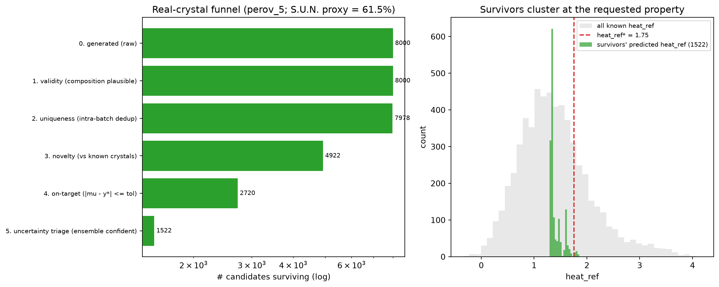
# ---- The discovery funnel + S.U.N.-style screening, on REAL crystals ----## Same six stages as Stage A, adapted to 118-dim composition space:## generate (wide top) -> raw candidate compositions# -> VALIDITY : a real composition: non-negative, sums to ~1, and at# least one element present (the deck's "physical# pre-filter" before any expensive screening)# -> UNIQUENESS: de-duplicate near-identical compositions (round the# fraction vector and drop repeats)# -> NOVELTY : far enough (L1 composition distance) from every KNOWN# crystal -> not a rediscovery# -> ON-TARGET : surrogate-predicted property within tol of the target# (we only ever get the SURROGATE, not true DFT, in a# real campaign)# -> UNCERTAINTY TRIAGE : keep only candidates the ensemble is confident# about (cross-tree sd below a data-driven cutoff) -- the# generative <-> UQ bridge, ensemble-flavoured## "S.U.N." = Stable . Unique . Novel; we report the surviving fraction# after the U+N stages (validity is the "stable/plausible" proxy here, as# in Stage A) and the final end-to-end yield.def discovery_funnel_crystals(cand, y_target, surrogate, X_known, novelty_tol=0.20, target_tol=None, sd_cutoff=None, verbose=True):"""Run the multi-stage funnel on 118-dim compositions.""" stages = [] x = np.asarray(cand, dtype=np.float64) stages.append(("0. generated (raw)", len(x)))# --- VALIDITY: non-negative, normalised (sum ~ 1), >=1 element. row = x.sum(axis=1) valid = (x >=0).all(axis=1) & (np.abs(row -1.0) <1e-6) &\ ((x >1e-6).sum(axis=1) >=1) x = x[valid] stages.append(("1. validity (composition plausible)", len(x)))# --- UNIQUENESS: round the fraction vector, drop intra-batch repeats.iflen(x): keys = np.round(x /0.02).astype(np.int64) _, uniq_idx = np.unique(keys, axis=0, return_index=True) x = x[np.sort(uniq_idx)] stages.append(("2. uniqueness (intra-batch dedup)", len(x)))# --- NOVELTY: min L1 composition distance to any KNOWN crystal.iflen(x):# chunked to keep the (n_cand x n_known) matrix small. keep = np.ones(len(x), dtype=bool)for s inrange(0, len(x), 512): blk = x[s:s +512] d = np.abs(blk[:, None, :] - X_known[None, :, :]).sum(axis=2) keep[s:s +512] = d.min(axis=1) > novelty_tol x = x[keep] stages.append(("3. novelty (vs known crystals)", len(x))) sun_rate =len(x) /max(stages[0][1], 1)# --- ON-TARGET: SURROGATE-predicted property near the target. mu_pred = sd_pred = np.array([])iflen(x): mu_pred, sd_pred = rf_mean_std(surrogate, x)if target_tol isNone:# tol = surrogate's own typical hold-out error scale: asking# for "within one surrogate-MAE of the target" (data-driven,# not an arbitrary constant). target_tol =max(mae_ho, 1e-6) on_t = np.abs(mu_pred - y_target) <= target_tol x, sd_pred = x[on_t], sd_pred[on_t] stages.append(("4. on-target (|mu - y*| <= tol)", len(x)))# --- UNCERTAINTY TRIAGE: ensemble must be confident. Cutoff is the# 60th-pct of the ensemble sd on the trusted HOLD-OUT crystals# (relative, exactly as Stage A calibrates against trusted points).iflen(x):if sd_cutoff isNone: sd_cutoff =float(np.percentile(sd_ho, 60)) x = x[sd_pred <= sd_cutoff] stages.append(("5. uncertainty triage (ensemble confident)", len(x)))if verbose:print(f" {'stage':<46s}{'#kept':>7s}{'frac':>9s}") n0 =max(stages[0][1], 1)for name, n in stages:print(f" {name:<46s}{n:>7d}{n / n0:>8.1%}")print(f" S.U.N. rate (Stable*Unique*Novel proxy) = {sun_rate:.1%}")print(f" end-to-end discovery yield = {len(x) / n0:.1%}")return x, stages, sun_rate# Wide top of funnel: over-generate, exactly as the deck insists.raw_cd = emulate_candidates(X_seed_cd, n_out=8000, jitter=0.15, seed=7)surv_cd, stage_cd, sun_cd = discovery_funnel_crystals( raw_cd, y_target_cd, surrogate_cd, X_seed_cd)
# Funnel waterfall (real crystals) + the property distribution of the# survivors vs the known set.fig, axes = plt.subplots(1, 2, figsize=(13, 5.2))ax = axes[0]labels = [s[0] for s in stage_cd]counts = [s[1] for s in stage_cd]ax.barh(range(len(counts)), np.maximum(counts, 1), color="#2ca02c")ax.set_yticks(range(len(labels)))ax.set_yticklabels(labels, fontsize=8)ax.invert_yaxis()ax.set_xscale("log")ax.set_xlabel("# candidates surviving (log)")ax.set_title(f"Real-crystal funnel (perov_5; S.U.N. proxy = {sun_cd:.1%})")for i, c inenumerate(counts): ax.text(max(c, 1), i, f" {c}", va="center", fontsize=8)ax = axes[1]ax.hist(y_cd, bins=40, alpha=0.5, color="lightgray", label=f"all known {target_col}")ax.axvline(y_target_cd, color="#d62728", ls="--", lw=1.5, label=f"{target_col}* = {y_target_cd:.2f}")iflen(surv_cd): mu_s, _ = rf_mean_std(surrogate_cd, surv_cd) ax.hist(mu_s, bins=20, alpha=0.7, color="#2ca02c", label=f"survivors' predicted {target_col} ({len(surv_cd)})")ax.set_xlabel(f"{target_col}")ax.set_ylabel("count")ax.set_title("Survivors cluster at the requested property")ax.legend(fontsize=8)plt.tight_layout()plt.show()
Read these two panels. Left: the identical deck funnel, now on real perovskite compositions — each stage trims the stream (log axis); the non-degenerate waterfall (survivors > 0, but a small fraction of the raw batch) is exactly the deck’s “wide top is mandatory, end-to-end yield is a fraction of a percent” picture, reproduced on real data rather than a 2-D toy. Right: the surviving candidates’ surrogate-predicted property concentrates around the requested target \(y^\star\), away from the bulk of the known distribution — inverse design on genuine crystals.
The braid, restated on real data. Stage A proved the mechanics (CVAE / classifier-free guidance) are legible in 2-D. Stage B proves the pipeline (funnel + S.U.N. + uncertainty triage) transfers verbatim to a real 118-dim generative-materials benchmark: only the surrogate (per-cluster GP → tree ensemble) and the substrate (E,H toy → CDVAE perovskites) changed; the generation-proposes / uncertainty-disposes logic is identical. That is the MFML × ML-PC × MG braid on the dataset the deck’s CDVAE→…→FlowMM models actually use.
Honest caveats (Stage B). (1) We do not train a 118-dim crystal generator — that is the deck’s SOTA and out of class scope; we emulate a generator’s output stream by composition-space jitter of real perovskites and screen it with the real funnel. (2) “Stable” is again a validity proxy (a plausible normalised composition), not an energy-above-hull computation against MP-2024/Alexandria; perov_5 has no hull column, which is itself the deck’s point that real S.U.N. needs a reference hull. (3) The composition features ignore structure (lattice/coordinates/space group) — real generators model those too — but the conditional-screening + UQ-triage logic this block teaches is structurally unchanged.
Block 7 — Student exercises
Three core (do all three) + two stretch (optional). Write your code in the empty cells below; bring printed plots / numbers to the next class for the 5-minute walk-through.
Exercise 1 (core) — Implement EI closed form from scratch
Block 3 used a closed-form Expected Improvement and we trusted the formula. Re-derive and reimplement it from \(\Phi\) and \(\phi\) alone, then verify it matches the version used above on a fixed test set.
Your task:
Implement \(\alpha_{\text{EI}}(x) = (\mu - f^* - \xi)\,\Phi(z) + \sigma\,\phi(z)\) with \(z = (\mu - f^* - \xi) / \sigma\), using only scipy.stats.norm.cdf and scipy.stats.norm.pdf (no other helpers).
Take 50 evenly-spaced strain values in \([0, 0.05]\). Predict \((\mu,
\sigma)\) from gp_recap.
Compute EI with your implementation and EI with acq_ei_factory(xi=0.01) from Block 3. Verify they agree to within 1e-10 numerically.
Plot EI(x) on the strain grid; mark the argmax with a vertical line.
Hint: be careful at \(\sigma = 0\) — set EI = 0 there (Block 3 does the same).
Exercise 2 (core) — Show that GP uncertainty is unreliable off-support
A GP with an RBF kernel has bounded uncertainty: outside the training data, the posterior mean reverts to the prior mean and the CI saturates at the prior amplitude \(\sigma_f\). This can be misleading: the CI says “I’m not sure” but with a fixed width that does not reflect how truly unconstrained the model is.
Your task:
Take TensileTestDataset(T=600). Train a GP only on the data points with strain \(x \in [0, 0.05]\).
Predict \((\mu, \sigma)\) at strains \(x \in [0, 0.5]\) — i.e., extrapolate 10x beyond the training range.
Plot the truth, the GP mean, and the 95% CI. Note where the CI fails to cover the truth.
Question (3 sentences in the markdown cell below). Why does the GP’s CI become unreliable here? Reference the stationarity of the RBF kernel.
Alternative framing if you finish quickly: instead of restricting the data range, fit a GP with a linear kernel on the same data and show how the resulting CI is miscalibrated against the reliability diagram from the homework.
(replace this text with your 3-sentence explanation)
Exercise 3 (core) — 2-D discovery threshold sweep
Block 5 used the median of pred_var and novelty as fixed thresholds. The result is a single (4-class) flag plot. The thresholds are arbitrary; in practice the metallurgist will tune them.
Your task:
Define a 2-D grid of thresholds: \(\tau_{\text{var}}\) at the 20/40/60/80 percentiles of pred_var, and \(\tau_{\text{nov}}\) at the 20/40/60/80 percentiles of novelty.
For each \((\tau_{\text{var}}, \tau_{\text{nov}})\) pair (16 pairs), count the number of “discovery candidates” (pred_var > tau_var AND novelty > tau_nov).
Plot a 4×4 heat map of the candidate counts. Annotate each cell.
Question (2 sentences). What is the trade-off? What does the metallurgist gain by lowering both thresholds, and what do they pay?
# TODO: your threshold-sweep heatmap goes here.# Skeleton:## pcts = [20, 40, 60, 80]# tau_vars = np.percentile(pred_var, pcts)# tau_novs = np.percentile(novelty, pcts)# heatmap = np.zeros((len(pcts), len(pcts)), dtype=int)# for i, tv in enumerate(tau_vars):# for j, tn in enumerate(tau_novs):# heatmap[i, j] = int(np.sum((pred_var > tv) & (novelty > tn)))# fig, ax = plt.subplots(figsize=(6, 5))# im = ax.imshow(heatmap, cmap="Reds", aspect="equal", origin="lower")# ...
Your answer to the trade-off question:
(replace this text with your 2-sentence explanation)
Exercise 4 (stretch) — Multi-fidelity GP with cheap-noisy + expensive-clean data
Real materials labs often have access to a cheap-noisy measurement (e.g. simulated stress-strain at T=600 with a coarse force model) and an expensive-clean measurement (e.g. real-rig stress-strain at T=0). A multi-fidelity GP combines them by treating the fidelity id as an extra input dimension and using a kernel of the form:
\[ k\big((x, f), (x', f')\big) \;=\; k_{\text{data}}(x, x') \cdot
\big(\,1 \text{ if } f = f' \text{ else } \rho\,\big), \]
where \(\rho \in [0, 1]\) is the cross-fidelity correlation. We fix \(\rho = 0.7\) for tractability; learning \(\rho\) jointly with the other kernel hyperparameters is a follow-up.
Your task:
Build a noisy variant of TensileTestDataset(T=600) by adding Gaussian noise of standard deviation 0.5 (in the standardised stress scale, or 50 MPa raw). Use 50 such cheap points.
Build a clean variant of TensileTestDataset(T=0) (use it as-is, sigma_n = 0.05). Use 10 such expensive points.
Fit three GPs:
only on the 50 cheap-noisy T=600 points,
only on the 10 clean T=0 points,
on both, with a fidelity-id input.
Plot RMSE on a held-out clean-T=600 set vs cumulative cost (cheap=1, expensive=5). The multi-fidelity GP should beat both single-fidelity baselines for some intermediate budget.
Hint: the simplest path is to concatenate (x, fidelity_id) as a 2-vector and let sklearn’s RBF kernel act on both dimensions. The “fidelity-aware” correlation \(\rho\) then comes from the lengthscale on the fidelity-id dimension — short lengthscale ≈ low cross-correlation, long lengthscale ≈ high cross-correlation. Hand-tune the fidelity-dim lengthscale so that points across fidelities still inform each other (a common choice is to set it to ~1.0 in standardised units).
Exercise 5 (stretch, optional) — Coverage under distribution shift
Block 4.5’s CQR construction gives a marginal-coverage guarantee only under exchangeability of calibration and test [@angelopoulos_2023_conformal]. Real materials labs routinely violate this: you calibrate UQ at one temperature, deploy at another, and the residual distribution shifts. This exercise shows the failure mode and two simple fixes.
Your task:
Train the Block 4.5 CQR pipeline (GP + quantile head + conformal correction \(\hat{Q}\)) only on TensileTestDataset(T=600) (warm conditions). Save the trained qhead, Q_hat, and gp_cqr.
Evaluate empirical coverage of the resulting intervals on TensileTestDataset(T=0) (cold conditions). It should drop well below the 0.9 target — typically to 0.6 or lower — even though the nominal target was 0.9. Exchangeability has failed.
Quick fix. Inflate \(\hat{Q}\) by a heuristic factor (e.g. 2x) and re-measure coverage on T=0. Note the coverage / width trade-off.
Principled fix: adaptive conformal. Implement the online update \(\hat\alpha_t \leftarrow \hat\alpha_{t-1} + \gamma\,(\mathbf{1}[\text{miss}_t] - \alpha)\) sweeping through the T=0 stream one sample at a time. After each step, recompute \(\hat{Q}_t\) as the \((1 - \hat\alpha_t)\)-quantile of the original calibration scores. Plot empirical coverage (cumulative or rolling-window) vs sample index. Show that the policy recovers to ~0.9 within a few hundred samples.
Hint: \(\gamma = 0.01\) is a fine default; set \(\hat\alpha_0 = \alpha\). Clip \(\hat\alpha_t\) to \((10^{-3}, 1 - 10^{-3})\) for stability.
Exercise 6 (stretch, optional) — Guidance weight vs the discovery funnel
Block 6.5 fixed the classifier-free-guidance weight at \(w=2\) for the funnel run and used median-based funnel cutoffs. CFG is the deck’s explicit fidelity ↔︎ diversity knob: cranking \(w\) pushes generated hardness onto the target but collapses diversity, which can starve the novelty stage of the funnel. This exercise quantifies that tension.
Your task:
For \(w \in \{0, 1, 2, 4, 8\}\), generate 5000 candidates at H_STAR with generate(cvae, H_STAR, n_samples=5000, guidance_w=w, seed=7).
Run each batch through discovery_funnel(..., verbose=False).
Plot, on a shared \(w\) axis: (a) the S.U.N. proxy rate, (b) the end-to-end discovery yield, and (c) the mean \(|H_{\text{gen}} - H^\star|\) of the raw batch (fidelity).
Question (3 sentences). Where is the sweet spot, and why does pushing \(w\) too high eventually reduce the number of synthesis-ready survivors even though on-target fidelity keeps improving?
Hint: reuse generate and discovery_funnel directly — no retraining. discovery_funnel already returns (survivors, stages, sun_rate).
# TODO: your guidance-weight sweep goes here.# Skeleton:## ws = [0, 1, 2, 4, 8]# sun_rates, yields, fidelities = [], [], []# for w in ws:# raw_w = generate(cvae, H_STAR, n_samples=5000, guidance_w=w, seed=7)# surv_w, _, sun_w = discovery_funnel(raw_w, H_STAR, sd_n, mu_n,# verbose=False)# sun_rates.append(sun_w)# yields.append(len(surv_w) / len(raw_w))# fidelities.append(float(np.abs(raw_w[:, 1] - H_STAR).mean()))# # plot the three curves vs ws ...
Your answer to the sweet-spot question:
(replace this text with your 3-sentence explanation)
Exam-aligned must-know statements (from MFML Unit 12 §“Exam-aligned”)
Re-read these after the exercises; today’s blocks have given you the concrete intuition for every one of them.
The GP posterior is a closed-form Gaussian: \(\mu^* = K_*^\top (K +
\sigma_n^2 I)^{-1} y\) and \(\Sigma^* = K_{**} - K_*^\top (K +
\sigma_n^2 I)^{-1} K_*\) (homework Part A; Block 1).
GP hyperparameters are learned by maximising the log marginal likelihood (homework Part A).
Deep ensembles and MC dropout are approximate GPs that scale better but lose calibration guarantees (homework Part B).
A reliability diagram measures empirical coverage vs nominal confidence — the operational test for whether a UQ method is trustworthy on your data (homework Part C).
Active learning queries the point with maximum predictive uncertainty (Block 2).
Acquisition functions trade off exploration (\(\sigma\)) and exploitation (\(\mu\)); UCB is robust, EI is the standard, PI over-exploits (Block 3).
Cost-aware AL replaces \(\alpha(x)\) with \(\alpha(x) / c(x)\) and is the simplest practical upgrade for real lab budgets (Block 4).
Discovery \(\neq\) labeling: a discovery candidate is simultaneously high predictive variance AND high novelty (Block 5).
Per-cluster acquisition budgets allow allocation strategies tuned to the objective (uniform fit vs maximum discovery) (Block 6).
Multi-fidelity GPs combine cheap-noisy and expensive-clean data and can beat either single-fidelity baseline for intermediate budgets (Block 7 stretch).
Exam-aligned must-know statements (from MG Unit 12 §“Key Takeaways”)
Inverse design = sampling from a learned conditional distribution \(p(x \mid y^\star)\), not searching \(\mathcal{X}\); the inverse problem is many-to-one and ill-posed (Block 6.5).
Conditional generation targets a property; unconditional samples the full data distribution and needs heavy filtering — conditioning quality dominates downstream success (Block 6.5).
Classifier-free guidance mixes the conditional and unconditional model (\(\tilde s = (1+w)\,s_{\text{cond}} - w\,s_{\text{uncond}}\)); \(w\) is the fidelity↔︎diversity knob (Block 6.5, Exercise 6).
Generated structures must pass the discovery funnel — validity → uniqueness → novelty → on-target → uncertainty triage — and S.U.N. (Stable/Unique/Novel) is reported as a rate; every stage trims by ~10–100× so the top of the funnel must be very wide (Block 6.5).
Uncertainty-aware filtering is the generative↔︎UQ bridge: the surrogate’s predictive variance decides which generated candidate is trustworthy enough for expensive validation (Block 6.5 — reuses the Block-5 per-cluster GP). Diffusion (CDVAE/DiffCSP/MatterGen) and flow (FlowMM) swap the decoder but keep this loop identical.