# Standard imports for the whole homework.
import numpy as np
import torch
import torch.nn as nn
import torch.nn.functional as F
import matplotlib.pyplot as plt

np.random.seed(0)
torch.manual_seed(0)
<torch._C.Generator at 0x7f30a8502270>This week braids three lectures’ Week 13 content onto one shared physics testbed — a damped harmonic oscillator with sparse, noisy observations.
Red thread. When you have a simulation model (an ODE, a PDE, an elastic limit) and a few noisy observations, you can build a regressor that is consistent with both. Today’s homework sets up the damped-oscillator testbed, fits a vanilla MLP that overfits the observations and ignores the physics, and adds an ODE residual to the loss — turning the MLP into a tiny PINN. Thursday will then add a GP baseline, an active-learning loop, and a real-materials elastic constraint on tensile data.
Time: ~75 minutes.
| Part | Min | Topic | Lecture anchor |
|---|---|---|---|
| A | 20 | Damped harmonic oscillator: closed-form solution + sparse noisy observations | MFML §“PINN setup” |
| B | 25 | Vanilla MLP regression on the sparse observations; show the physics-blind overfit | MFML §“why physics-only constraints help”; ML-PC §“failure modes of unconstrained models” |
| C | 20 | Add the ODE residual to the loss → tiny PINN; re-train; compare | MFML §“PINN auto-diff residual” |
| D | 10 | Reflection: when does a physics constraint help, when does it hurt, and what happens when the physics is wrong? | bridge to Thursday |
# Standard imports for the whole homework.
import numpy as np
import torch
import torch.nn as nn
import torch.nn.functional as F
import matplotlib.pyplot as plt
np.random.seed(0)
torch.manual_seed(0)<torch._C.Generator at 0x7f30a8502270>We work with the simplest non-trivial second-order linear ODE: \[ m \ddot x + \gamma \dot x + k\, x = 0, \qquad x(0) = 1,\ \dot x(0) = 0. \] With \(m = 1\), \(k = 1\), and a small damping \(\gamma = 0.3\) the system is underdamped, and the closed-form solution is \[ x(t) = e^{-\gamma t/2} \cos(\omega_d t), \qquad \omega_d = \sqrt{k/m - \gamma^2/4}. \] This is our ground truth. We sample 7 sparse, noisy observations of \(x(t)\) over \(t \in [0, 20]\) — the “experimental measurements” we have to work with. The full continuous trajectory is unknown to the model.
M, K_SP, GAMMA = 1.0, 1.0, 0.3
omega_d = np.sqrt(K_SP / M - (GAMMA / 2.0) ** 2)
T_MAX = 20.0


def true_x(t):
    """Closed-form underdamped solution with x(0)=1, x'(0)=0."""
    return np.exp(-GAMMA * t / 2.0) * np.cos(omega_d * t)


# 7 sparse observation points + Gaussian noise on the measurement.
rng = np.random.default_rng(0)
t_obs = np.array([0.5, 2.5, 4.5, 7.5, 11.5, 15.0, 18.0])
NOISE_SIGMA = 0.05
x_obs = true_x(t_obs) + rng.normal(0, NOISE_SIGMA, size=t_obs.shape)

# Dense grid for plotting (NOT used as training data).
t_dense = np.linspace(0, T_MAX, 400)
x_true_dense = true_x(t_dense)

print(f"Part A — damped oscillator setup:")
print(f"  m = {M}, k = {K_SP}, gamma = {GAMMA}")
print(f"  omega_d = sqrt(k/m - gamma^2/4) = {omega_d:.4f}  rad/s")
print(f"  observed times: {t_obs}")
print(f"  observation noise sigma: {NOISE_SIGMA}")
Part A — damped oscillator setup:
m = 1.0, k = 1.0, gamma = 0.3
omega_d = sqrt(k/m - gamma^2/4) = 0.9887 rad/s
observed times: [ 0.5 2.5 4.5 7.5 11.5 15. 18. ]
observation noise sigma: 0.05fig, ax = plt.subplots(figsize=(8, 4.5))
ax.plot(t_dense, x_true_dense, "k-", lw=1.5, label="analytic $x(t)$")
ax.errorbar(t_obs, x_obs, yerr=NOISE_SIGMA, fmt="o", color="tab:red",
ms=7, capsize=3, label="7 noisy observations")
ax.set_xlabel("$t$ (s)")
ax.set_ylabel("$x(t)$")
ax.set_title("Part A — damped harmonic oscillator: ground truth + sparse data")
ax.grid(alpha=0.3)
ax.legend()
plt.tight_layout()
plt.show()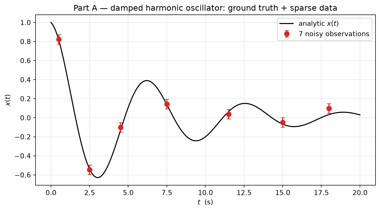
Part A deliverable: the plot above. Notice how few points we have relative to the oscillation: between \(t=4.5\) and \(t=7.5\) we have zero data, yet the analytic solution oscillates through a full period in that gap. Any model that only sees the points has no way to know about the oscillation in that interval — unless it also sees the physics.
Fit a small MLP to the 7 noisy observations with plain MSE loss, no physics. The model has no idea what \(\gamma\), \(k\), or \(\omega_d\) are. It will fit the observations exactly and produce nonsense between them.
class MLP(nn.Module):
    def __init__(self, hidden: int = 32, depth: int = 3):
        super().__init__()
        layers = [nn.Linear(1, hidden), nn.Tanh()]
        for _ in range(depth - 1):
            layers += [nn.Linear(hidden, hidden), nn.Tanh()]
        layers += [nn.Linear(hidden, 1)]
        self.net = nn.Sequential(*layers)

    def forward(self, t):
        return self.net(t).squeeze(-1)


t_obs_t = torch.tensor(t_obs, dtype=torch.float32).unsqueeze(-1)
x_obs_t = torch.tensor(x_obs, dtype=torch.float32)
t_dense_t = torch.tensor(t_dense, dtype=torch.float32).unsqueeze(-1)

torch.manual_seed(0)
mlp_vanilla = MLP()
opt = torch.optim.Adam(mlp_vanilla.parameters(), lr=5e-3)

n_epochs = 4000
for ep in range(n_epochs):
    opt.zero_grad()
    pred = mlp_vanilla(t_obs_t)
    loss = F.mse_loss(pred, x_obs_t)
    loss.backward()
    opt.step()

mlp_vanilla.eval()
with torch.no_grad():
    x_pred_vanilla = mlp_vanilla(t_dense_t).numpy()
rmse_vanilla = float(np.sqrt(np.mean((x_pred_vanilla - x_true_dense) ** 2)))
print(f"Part B — vanilla MLP after {n_epochs} epochs:")
print(f"  training MSE on 7 observations: {F.mse_loss(mlp_vanilla(t_obs_t), x_obs_t).item():.6f}")
print(f"  RMSE on dense grid (vs analytic): {rmse_vanilla:.4f}")
Part B — vanilla MLP after 4000 epochs:
training MSE on 7 observations: 0.000566
RMSE on dense grid (vs analytic): 0.2040fig, ax = plt.subplots(figsize=(9, 5))
ax.plot(t_dense, x_true_dense, "k-", lw=1.5, label="analytic $x(t)$")
ax.errorbar(t_obs, x_obs, yerr=NOISE_SIGMA, fmt="o", color="tab:red",
ms=7, capsize=3, label="observations")
ax.plot(t_dense, x_pred_vanilla, "b--", lw=2, label="vanilla MLP")
ax.set_xlabel("$t$ (s)")
ax.set_ylabel("$x(t)$")
ax.set_title(f"Part B — vanilla MLP: physics-blind (grid RMSE = {rmse_vanilla:.3f})")
ax.grid(alpha=0.3); ax.legend()
plt.tight_layout()
plt.show()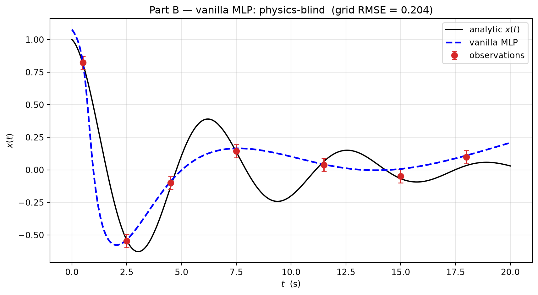
Part B deliverable: the figure and the printed RMSE.
What goes wrong:
A PINN encodes the governing ODE directly in the loss. We add a residual term \[
\mathcal{L}_\text{phys}(\theta) = \frac{1}{N_c}\sum_{i=1}^{N_c}\!\left[m\,\ddot x_\theta(t_i^c) + \gamma\,\dot x_\theta(t_i^c) + k\,x_\theta(t_i^c)\right]^2,
\] evaluated at \(N_c\) collocation points \(t_i^c\) that span the domain (no observations needed at those points). The derivatives are computed with torch.autograd.grad — the model is differentiable, so this is a one-liner. The total loss is \[
\mathcal{L} = \mathcal{L}_\text{data} + \lambda\, \mathcal{L}_\text{phys}.
\] We also add the boundary conditions \(x(0) = 1\), \(\dot x(0) = 0\) as a tiny additional MSE term — three numbers we know without measurement.
def ode_residual(model, t_collocation):
    """Return m*x'' + gamma*x' + k*x evaluated at collocation points."""
    t = t_collocation.requires_grad_(True)
    x = model(t)
    dxdt = torch.autograd.grad(x.sum(), t, create_graph=True)[0]
    d2xdt2 = torch.autograd.grad(dxdt.sum(), t, create_graph=True)[0]
    return M * d2xdt2 + GAMMA * dxdt + K_SP * x


# Collocation points: 200 evenly spaced t in [0, 20]. NO measurements here.
t_coll = torch.linspace(0, T_MAX, 200, dtype=torch.float32).unsqueeze(-1)
t_zero = torch.zeros(1, 1, dtype=torch.float32, requires_grad=True)

torch.manual_seed(0)
pinn = MLP()
opt = torch.optim.Adam(pinn.parameters(), lr=5e-3)

LAMBDA_PHYS = 1.0
LAMBDA_BC = 1.0
n_epochs = 4000
for ep in range(n_epochs):
    opt.zero_grad()

    # Data loss (the 7 noisy observations).
    loss_data = F.mse_loss(pinn(t_obs_t), x_obs_t)

    # Physics loss (collocation residuals; no labels needed).
    res = ode_residual(pinn, t_coll)
    loss_phys = (res ** 2).mean()

    # Boundary conditions: x(0) = 1, x'(0) = 0.
    x0 = pinn(t_zero)
    dxdt0 = torch.autograd.grad(x0.sum(), t_zero, create_graph=True)[0]
    loss_bc = (x0 - 1.0).pow(2).mean() + dxdt0.pow(2).mean()

    loss = loss_data + LAMBDA_PHYS * loss_phys + LAMBDA_BC * loss_bc
    loss.backward()
    opt.step()

pinn.eval()
with torch.no_grad():
    x_pred_pinn = pinn(t_dense_t).numpy()
rmse_pinn = float(np.sqrt(np.mean((x_pred_pinn - x_true_dense) ** 2)))
print(f"Part C — PINN after {n_epochs} epochs (lambda_phys = {LAMBDA_PHYS}, lambda_bc = {LAMBDA_BC}):")
print(f"  data MSE:    {F.mse_loss(pinn(t_obs_t), x_obs_t).item():.6f}")
print(f"  phys MSE:    {(ode_residual(pinn, t_coll) ** 2).mean().item():.6f}")
print(f"  RMSE on dense grid (vs analytic): {rmse_pinn:.4f}")
print(f"  vanilla / PINN improvement factor: {rmse_vanilla / rmse_pinn:.1f}x")
Part C — PINN after 4000 epochs (lambda_phys = 1.0, lambda_bc = 1.0):
data MSE: 0.018516
phys MSE: 0.042269
RMSE on dense grid (vs analytic): 0.1721
vanilla / PINN improvement factor: 1.2xfig, ax = plt.subplots(figsize=(9, 5))
ax.plot(t_dense, x_true_dense, "k-", lw=1.5, label="analytic $x(t)$")
ax.errorbar(t_obs, x_obs, yerr=NOISE_SIGMA, fmt="o", color="tab:red",
ms=7, capsize=3, label="observations")
ax.plot(t_dense, x_pred_vanilla, "b--", lw=2, alpha=0.7,
label=f"vanilla MLP (RMSE {rmse_vanilla:.3f})")
ax.plot(t_dense, x_pred_pinn, "g-", lw=2,
label=f"PINN (RMSE {rmse_pinn:.3f})")
ax.set_xlabel("$t$ (s)")
ax.set_ylabel("$x(t)$")
ax.set_title("Part C — PINN matches the physics in regions with no data")
ax.grid(alpha=0.3); ax.legend()
plt.tight_layout()
plt.show()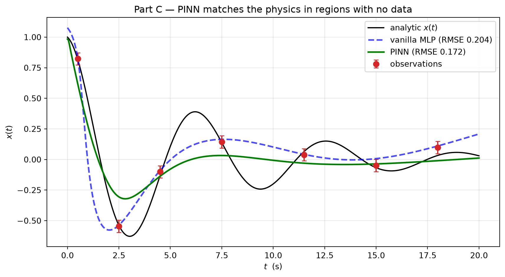
Part C deliverable: the comparison figure above and the printed RMSE improvement factor.
What changed:
The PINN beats the vanilla MLP because the physics is correct. But what happens when the physics encoded in the loss is wrong? Thursday Block 7 will demonstrate this in code, but think it through now.
Your task (~10 min, write 4-6 sentences):
Pick one materials scenario and answer two questions:
Bring the paragraph to Thursday; we will pick two volunteers to read theirs aloud at the start of Block 1.
Hand in: your written paragraph (Markdown cell below).
(your reflection paragraph here)