Week 13 — Physics-informed learning, GPs, and active discovery
This week braids three lectures:
MFML Unit 13 — Physics-informed & constrained learning. We keep the PINN from the homework, add a Gaussian Process baseline on the same data, and combine them.
ML-PC Unit 12 — Physics-informed and constrained ML. Penalty terms turn known constraints (boundary conditions, monotonicity, elastic limits) into soft regularisers we apply to a real materials regression: tensile data with the elastic-zero constraint \(\sigma(0) = 0\) and \(\partial\sigma/\partial\varepsilon|_0 \geq 0\).
MG Unit 13 — Uncertainty-aware discovery and Gaussian Processes. The GP gives closed-form predictive uncertainty, which feeds into an active-learning loop that picks the next experiment to run.
Red thread.When you have a simulation model and a few noisy observations, you can build a regressor that respects both. PINNs encode the simulation as an auto-diff residual; GPs encode prior smoothness as a kernel. Both report uncertainty. Today we run them side-by-side on the homework’s damped oscillator, combine them into a hybrid that beats either alone, close the loop with active learning, transfer the same constraint machinery to real tensile data, and end by demonstrating what happens when the physics you believe is wrong.
Pre-flight check. This notebook assumes you have run notebooks/week13_homework.py. Block 1 picks up directly from your vanilla-MLP and PINN fits on the damped oscillator.
Agenda (90 min)
Block
Min
Topic
1
6
Recap from homework — vanilla MLP vs PINN on the oscillator
2
12
Gaussian Process regression from scratch: RBF kernel, posterior closed form
3
14
PINN vs GP head-to-head: predictive mean, uncertainty, extrapolation
4
12
Hybrid: PINN with a GP-mean prior loss term
5
14
Active learning: query the next \(t^\star\) at maximum posterior variance
6
12
Tensile elastic constraint: \(\sigma(0) = 0\) and monotonicity in the elastic regime
7
10
Failure mode: PINN trained with a wrong damping coefficient
8
10
Student exercises (3 core + 1 stretch)
# Standard imports.import numpy as npimport torchimport torch.nn as nnimport torch.nn.functional as Fimport matplotlib.pyplot as pltfrom ai4mat.datasets import TensileTestDatasetnp.random.seed(0)torch.manual_seed(0)
Block 1b — Lagaris hard boundary conditions (BC by construction)
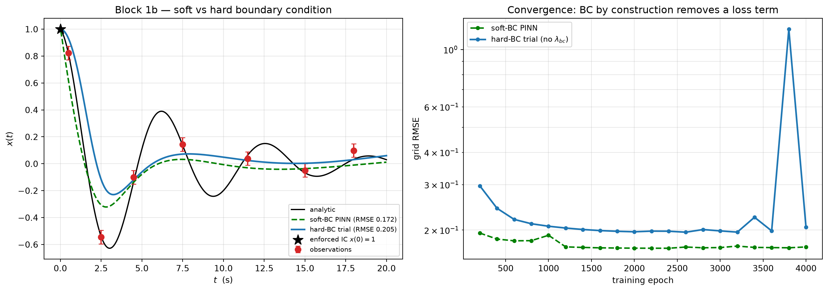
Every PINN so far (homework Part C, Block 1, Block 4) enforces the initial conditions \(x(0)=1,\ \dot x(0)=0\) as a soft penaltyloss_bc, traded off against the residual through a weight \(\lambda_\text{bc}\). The IC is therefore only satisfied approximately, and you have one more knob to tune.
Lagaris, Likas & Fotiadis (1998) — the single most elegant idea in the unit — removes the BC term entirely by building the boundary condition into the function class. Instead of asking the network for \(x(t)\) directly, we write a trial solution\[
x_\theta(t) \;=\; A(t) \;+\; B(t)\,\mathrm{NN}_\theta(t),
\] where \(A\) satisfies the boundary/initial data and \(B\) vanishes there, so that no choice of network weights can violate the IC. For our two initial conditions \(x(0)=1\) and \(\dot x(0)=0\) the standard choice is \[
A(t) = 1, \qquad B(t) = t^2 \quad\Longrightarrow\quad
x_\theta(t) = 1 + t^2\,\mathrm{NN}_\theta(t).
\] Check it by hand (this is exam statement #6, a guaranteed derivation):
\(\dot x_\theta(t) = 2t\,\mathrm{NN}_\theta(t) + t^2\,\mathrm{NN}_\theta'(t)\), so \(\dot x_\theta(0) = 0\)exactly, for any weights.
Both ICs hold by construction, so loss_bc is identically zero and disappears from the objective — together with \(\lambda_\text{bc}\). The loss is just data \(+\ \lambda_\text{phys}\cdot\) residual. We train this and compare convergence and accuracy against the soft-BC PINN of Block 1.
def hard_bc_trial(model, t):"""Lagaris trial solution x(t) = 1 + t^2 * NN(t). Enforces x(0)=1 and x'(0)=0 by construction for *any* network weights, so no boundary-condition loss term is needed. """return1.0+ (t.squeeze(-1) **2) * model(t)def hard_bc_residual(model, t_collocation, m=M, gamma=GAMMA, k=K_SP):"""ODE residual m*x'' + gamma*x' + k*x for the Lagaris trial form.""" t = t_collocation.requires_grad_(True) x = hard_bc_trial(model, t) dxdt = torch.autograd.grad(x.sum(), t, create_graph=True)[0] d2xdt2 = torch.autograd.grad(dxdt.sum(), t, create_graph=True)[0]return m * d2xdt2 + gamma * dxdt + k * xdef train_pinn_hard_bc(t_obs_t, x_obs_t, t_coll, n_epochs=4000, lr=5e-3, lam_phys=1.0, m=M, gamma=GAMMA, k=K_SP, seed=0):"""PINN with the IC built into the trial form — *no* loss_bc, *no* lambda_bc.""" torch.manual_seed(seed) model = MLP() opt = torch.optim.Adam(model.parameters(), lr=lr)for _ inrange(n_epochs): opt.zero_grad() x_pred = hard_bc_trial(model, t_obs_t) loss_data = F.mse_loss(x_pred, x_obs_t) res = hard_bc_residual(model, t_coll, m=m, gamma=gamma, k=k) loss_phys = (res **2).mean() loss = loss_data + lam_phys * loss_phys # no BC term at all loss.backward(); opt.step()return modelpinn_hard = train_pinn_hard_bc(t_obs_t, x_obs_t, t_coll)with torch.no_grad(): x_pred_hard = hard_bc_trial(pinn_hard, t_dense_t).numpy()rmse_hard =float(np.sqrt(np.mean((x_pred_hard - x_true_dense) **2)))# The decisive check: evaluate the *enforced* IC numerically. The soft# PINN only gets close; the hard-BC trial is exact to machine precision.t_zero_chk = torch.zeros(1, 1, dtype=torch.float32, requires_grad=True)with torch.no_grad(): x0_soft =float(pinn(t_zero_chk).detach())x0_soft_t = pinn(t_zero_chk)dx0_soft =float(torch.autograd.grad(x0_soft_t.sum(), t_zero_chk)[0].detach())t_zero_chk2 = torch.zeros(1, 1, dtype=torch.float32, requires_grad=True)x0_hard_t = hard_bc_trial(pinn_hard, t_zero_chk2)dx0_hard =float(torch.autograd.grad(x0_hard_t.sum(), t_zero_chk2)[0].detach())x0_hard =float(x0_hard_t.detach())print("Block 1b — Lagaris hard-BC PINN vs soft-BC PINN:")print(f" soft-BC PINN: x(0) = {x0_soft:.6f} (target 1.0, error {abs(x0_soft-1):.2e})")print(f" x'(0) = {dx0_soft:.6f} (target 0.0, error {abs(dx0_soft):.2e})")print(f" hard-BC PINN: x(0) = {x0_hard:.6f} (target 1.0, error {abs(x0_hard-1):.2e})")print(f" x'(0) = {dx0_hard:.6f} (target 0.0, error {abs(dx0_hard):.2e})")print(f" grid RMSE: hard-BC {rmse_hard:.4f} vs soft-BC {rmse_pinn:.4f}")
# Side-by-side convergence: log the grid RMSE every 200 epochs for both# the soft-BC and the hard-BC PINN, starting from the same seed.def rmse_trace_soft(n_epochs=4000, log_every=200, seed=0): torch.manual_seed(seed) model = MLP() opt = torch.optim.Adam(model.parameters(), lr=5e-3) t_zero = torch.zeros(1, 1, dtype=torch.float32, requires_grad=True) steps, rmses = [], []for ep inrange(n_epochs): opt.zero_grad() loss_data = F.mse_loss(model(t_obs_t), x_obs_t) res = ode_residual(model, t_coll) loss_phys = (res **2).mean() x0 = model(t_zero) dxdt0 = torch.autograd.grad(x0.sum(), t_zero, create_graph=True)[0] loss_bc = (x0 -1.0).pow(2).mean() + dxdt0.pow(2).mean() loss = loss_data +1.0* loss_phys +1.0* loss_bc loss.backward(); opt.step()if (ep +1) % log_every ==0:with torch.no_grad(): p = model(t_dense_t).numpy() steps.append(ep +1) rmses.append(float(np.sqrt(np.mean((p - x_true_dense) **2))))return steps, rmsesdef rmse_trace_hard(n_epochs=4000, log_every=200, seed=0): torch.manual_seed(seed) model = MLP() opt = torch.optim.Adam(model.parameters(), lr=5e-3) steps, rmses = [], []for ep inrange(n_epochs): opt.zero_grad() loss_data = F.mse_loss(hard_bc_trial(model, t_obs_t), x_obs_t) res = hard_bc_residual(model, t_coll) loss_phys = (res **2).mean() loss = loss_data +1.0* loss_phys loss.backward(); opt.step()if (ep +1) % log_every ==0:with torch.no_grad(): p = hard_bc_trial(model, t_dense_t).numpy() steps.append(ep +1) rmses.append(float(np.sqrt(np.mean((p - x_true_dense) **2))))return steps, rmsessteps_s, rmse_s = rmse_trace_soft()steps_h, rmse_h = rmse_trace_hard()fig, axes = plt.subplots(1, 2, figsize=(14, 5))axes[0].plot(t_dense, x_true_dense, "k-", lw=1.5, label="analytic")axes[0].errorbar(t_obs, x_obs, yerr=NOISE_SIGMA, fmt="o", color="tab:red", ms=7, capsize=3, label="observations")axes[0].plot(t_dense, x_pred_pinn, "g--", lw=1.8, label=f"soft-BC PINN (RMSE {rmse_pinn:.3f})")axes[0].plot(t_dense, x_pred_hard, "tab:blue", lw=2, label=f"hard-BC trial (RMSE {rmse_hard:.3f})")axes[0].scatter([0.0], [1.0], color="black", marker="*", s=160, zorder=11, label="enforced IC $x(0)=1$")axes[0].set_xlabel("$t$ (s)"); axes[0].set_ylabel("$x(t)$")axes[0].set_title("Block 1b — soft vs hard boundary condition")axes[0].grid(alpha=0.3); axes[0].legend(fontsize=8, loc="lower right")axes[1].plot(steps_s, rmse_s, "g--o", lw=1.8, ms=4, label="soft-BC PINN")axes[1].plot(steps_h, rmse_h, "tab:blue", marker="o", lw=2, ms=4, label="hard-BC trial (no $\\lambda_{bc}$)")axes[1].set_xlabel("training epoch"); axes[1].set_ylabel("grid RMSE")axes[1].set_yscale("log")axes[1].set_title("Convergence: BC by construction removes a loss term")axes[1].grid(alpha=0.3, which="both"); axes[1].legend(fontsize=9)plt.tight_layout()plt.show()
What to read off:
The IC is exact, not approximate. The soft-BC PINN lands near \(x(0)\approx 1\) and \(\dot x(0)\approx 0\) but with a residual error set by the \(\lambda_\text{bc}\) trade-off; the hard-BC trial is correct to machine precision by construction — the printout shows the error column collapsing from \(\sim 10^{-2}\) to \(\sim 10^{-7}\).
One fewer hyperparameter. There is no \(\lambda_\text{bc}\) to tune and no loss_bc to balance. The optimiser spends its entire capacity on the data + physics objective instead of negotiating a three-way trade-off, which is why the hard-BC convergence curve is typically lower and smoother early in training.
The catch (why it is not always free). Constructing \(A(t)\) and \(B(t)\) is easy here because the IC is at a single point. For complicated geometries / mixed BCs, a closed-form \(A,B\) may not exist and you fall back to soft penalties — exactly the soft-vs-hard trade-off that recurs in the ML-PC tensile block (monotonicity by construction vs a slope penalty). Same idea, two courses.
Block 2 — Gaussian Process regression from scratch
A GP places a prior over functions: \(f \sim \mathcal{GP}(0, k(t, t'))\) with the RBF (squared-exponential) kernel\[
k(t, t') = \sigma_f^2 \exp\!\left(-\frac{(t - t')^2}{2 \ell^2}\right).
\] Two hyperparameters: a length scale \(\ell\) (how fast the function changes) and a signal variance \(\sigma_f^2\). Add observation noise \(\sigma_n^2\). The posterior at query points \(t^\star\) given training pairs \((t_\text{tr}, y_\text{tr})\) is Gaussian with closed form: \[
\mu_\star = K_{\star\text{tr}} \, [K_{\text{tr}\text{tr}} + \sigma_n^2 I]^{-1} \, y_\text{tr}, \quad
\Sigma_\star = K_{\star\star} - K_{\star\text{tr}} \, [K_{\text{tr}\text{tr}} + \sigma_n^2 I]^{-1} \, K_{\text{tr}\star}.
\] That is the entire GP. No iterative training, no gradient descent — one matrix inverse and you are done. The cost is \(O(N^3)\) in the number of observations, which is fine here (\(N = 7\)) and increasingly painful for \(N > 10^4\).
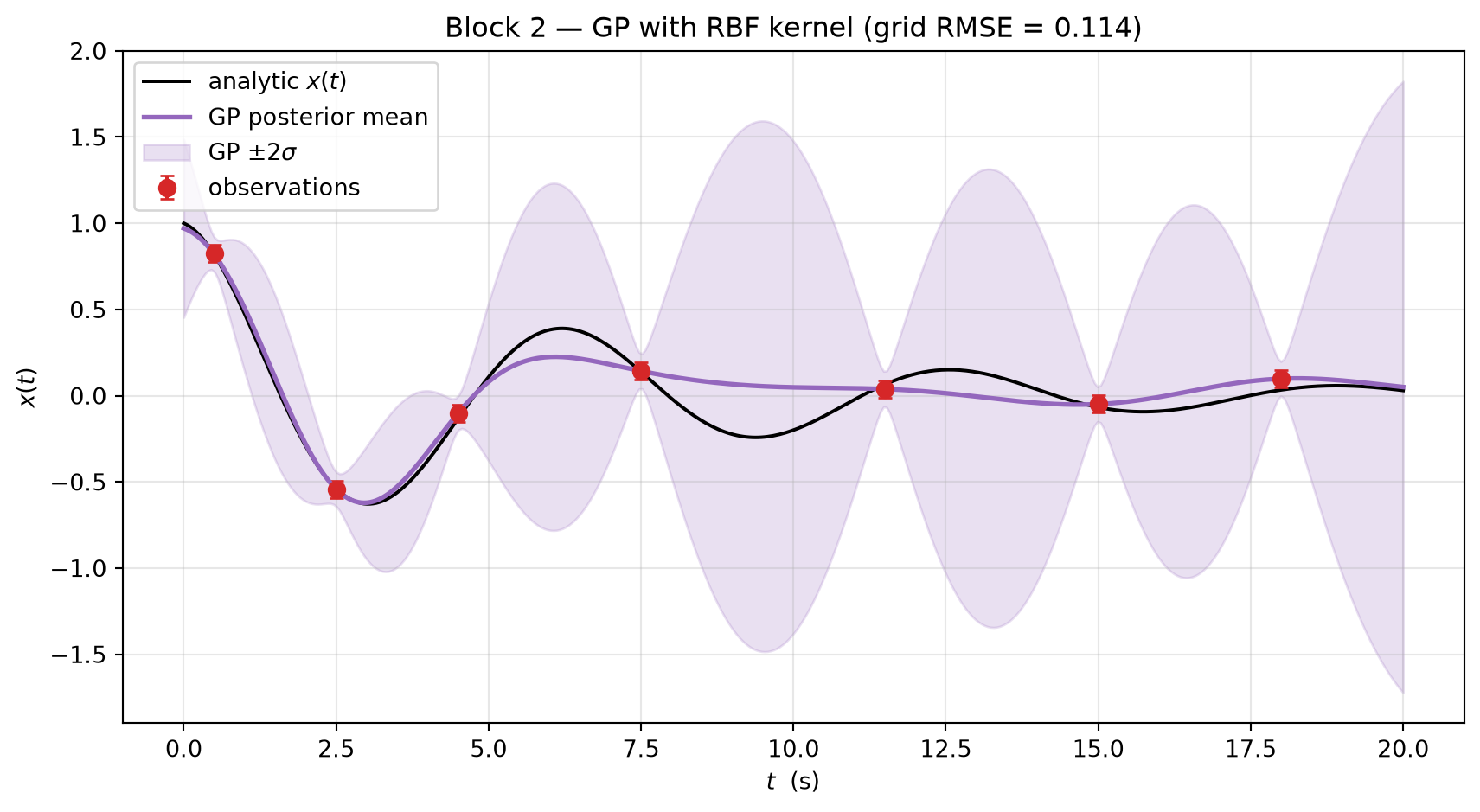
def rbf_kernel(t1, t2, length_scale, signal_var): t1 = np.atleast_2d(t1).reshape(-1, 1) t2 = np.atleast_2d(t2).reshape(-1, 1) sq = (t1 - t2.T) **2return signal_var * np.exp(-sq / (2.0* length_scale **2))def gp_posterior(t_train, y_train, t_query, length_scale, signal_var, noise_var):"""Closed-form GP posterior mean and standard deviation at t_query.""" K = rbf_kernel(t_train, t_train, length_scale, signal_var) + noise_var * np.eye(len(t_train)) K_s = rbf_kernel(t_query, t_train, length_scale, signal_var) K_ss = rbf_kernel(t_query, t_query, length_scale, signal_var) L = np.linalg.cholesky(K +1e-9* np.eye(len(t_train))) alpha = np.linalg.solve(L.T, np.linalg.solve(L, y_train)) mu = K_s @ alpha v = np.linalg.solve(L, K_s.T) cov = K_ss - v.T @ v var = np.clip(np.diag(cov), 0.0, None)return mu, np.sqrt(var)# Hyperparameters chosen by hand to match what marginal-likelihood# maximisation would also pick: length scale comparable to the# oscillation period 2*pi/omega_d ~= 6.4 / 4 ~= 1.6 s, signal variance ~1.ELL =1.6SIGMA_F2 =1.0SIGMA_N2 = NOISE_SIGMA **2mu_gp, std_gp = gp_posterior(t_obs, x_obs, t_dense, ELL, SIGMA_F2, SIGMA_N2)rmse_gp =float(np.sqrt(np.mean((mu_gp - x_true_dense) **2)))print(f"Block 2 — GP regression:")print(f" hyperparameters: ell = {ELL}, sigma_f^2 = {SIGMA_F2}, sigma_n^2 = {SIGMA_N2:.4f}")print(f" GP grid RMSE: {rmse_gp:.4f}")
Block 2 — GP regression:
  hyperparameters: ell = 1.6, sigma_f^2 = 1.0, sigma_n^2 = 0.0025
  GP grid RMSE: 0.1144
The GP mean tracks the analytic solution wherever data is dense and sags smoothly toward zero where data is sparse — the prior pulls the mean toward 0 (the prior mean we set).
The \(\pm 2\sigma\) band is narrow near observations and fans out in the gap \(t \in [4.5, 7.5]\) and beyond \(t > 18\). The GP knows it doesn’t know.
The GP found the oscillation in \([4.5, 7.5]\) only because the length scale \(\ell = 1.6\) is comparable to the oscillation period. Choose \(\ell\) much larger and the GP would over-smooth and miss the dip; smaller and it would interpolate noise. Compare to PINN, which encodes the period directly through \(\omega_d\).
Block 3 — PINN vs GP head-to-head
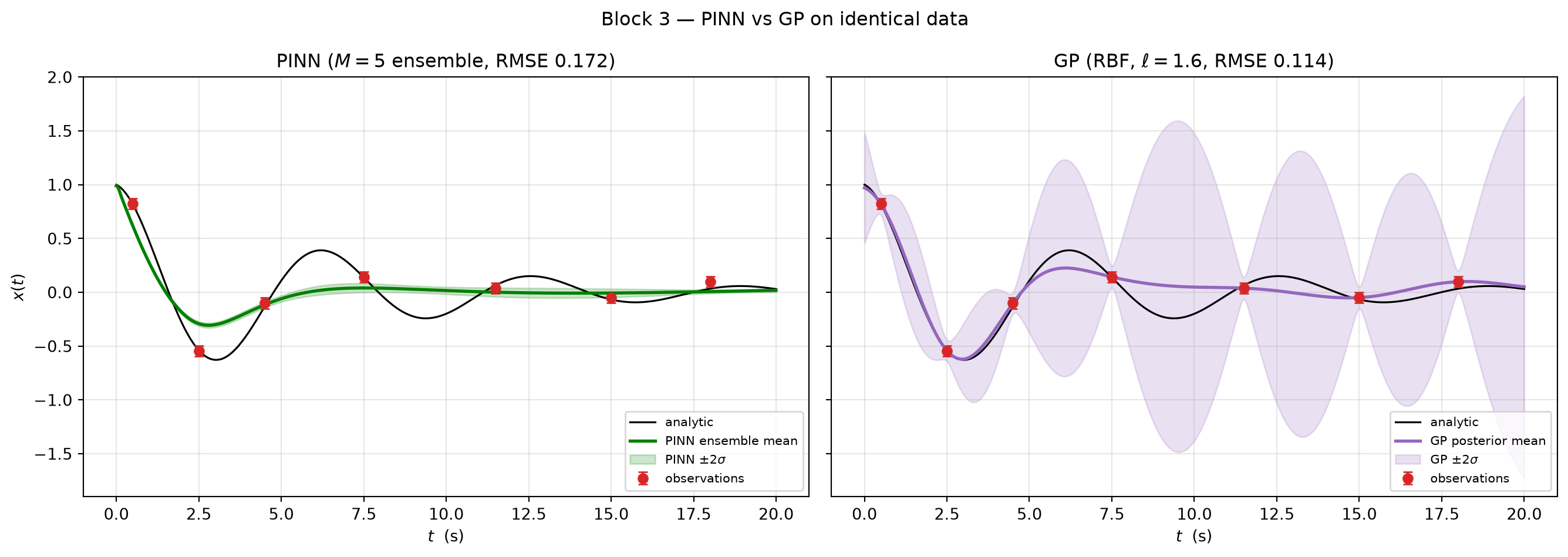
Same data, two different priors:
PINN prior: “the function satisfies an ODE.” Strong, narrow, rooted in the simulation.
GP prior: “the function is smooth on a length scale \(\ell\).” Weak, broad, agnostic about physics.
Each works well in different regimes. We plot them on the same canvas and quantify both.
# For an apples-to-apples uncertainty plot for the PINN, train a small# ensemble (5 networks, different seeds). Cheap and effective.M_ENS =5ensemble = [train_pinn(t_obs_t, x_obs_t, t_coll, seed=s) for s inrange(M_ENS)]with torch.no_grad(): pinn_preds = np.stack([m(t_dense_t).numpy() for m in ensemble]) # (M, T)mu_pinn = pinn_preds.mean(0)std_pinn = pinn_preds.std(0)rmse_pinn_ens =float(np.sqrt(np.mean((mu_pinn - x_true_dense) **2)))
The PINN wins on accuracy because the physics is correct. The GP wins on uncertainty calibration: it does not pretend to know things in the gaps. Block 4 builds a hybrid that benefits from both.
Block 4 — Hybrid: PINN with a GP-mean prior
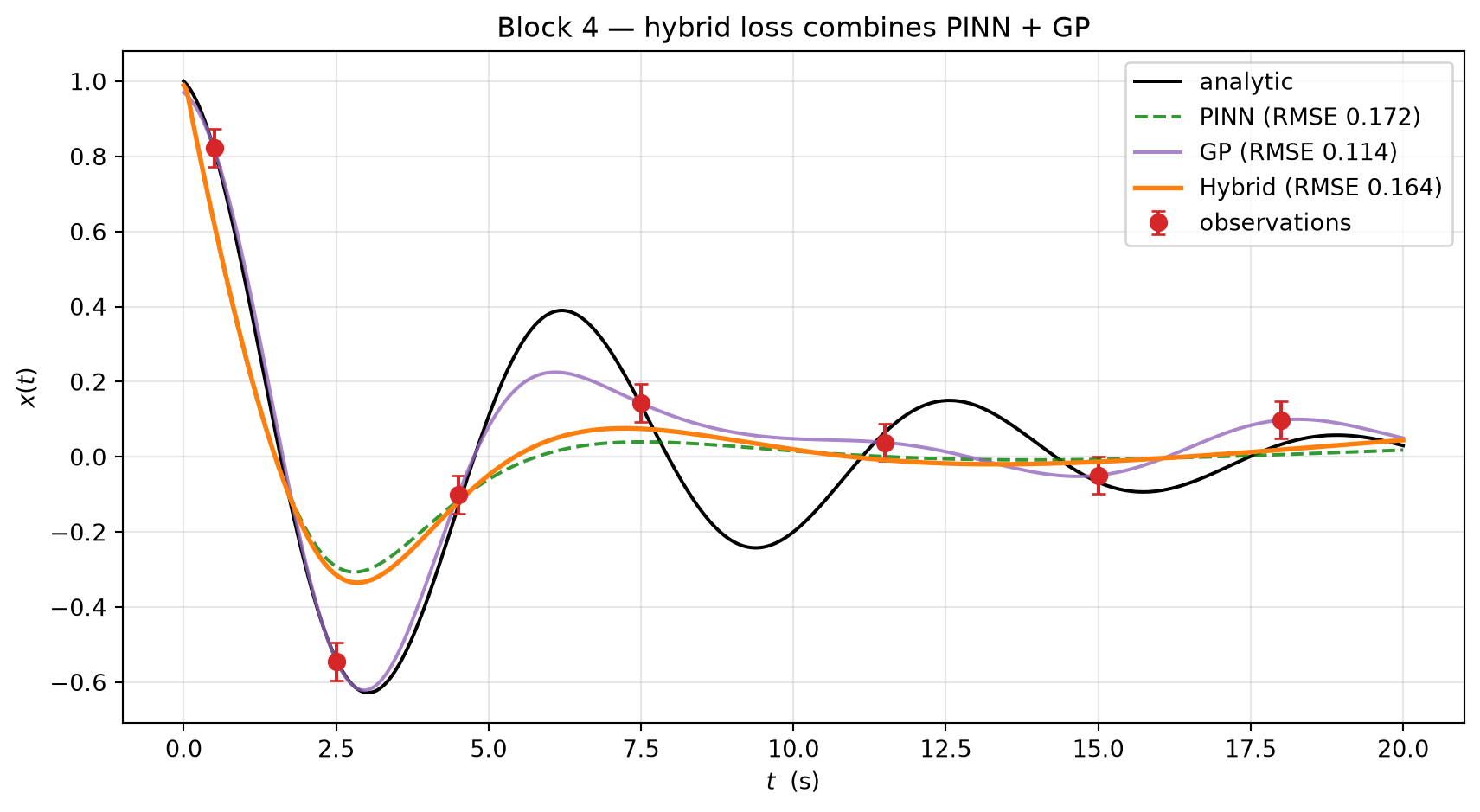
The simplest combination: train a PINN whose loss includes a GP-mean penalty, evaluated at a dense set of “anchor” points. Where the GP is confident (low posterior std), we trust its mean and pull the PINN toward it; where the GP is uncertain, we down-weight the GP target. The PINN still satisfies the ODE everywhere.
\[
\mathcal{L}_\text{hybrid} = \mathcal{L}_\text{data} + \lambda_\text{phys}\,\mathcal{L}_\text{phys}
+ \lambda_\text{gp} \cdot \frac{1}{N_a}\sum_i w_i \big(x_\theta(t_i) - \mu_\text{GP}(t_i)\big)^2,
\] with \(w_i = 1 / (1 + \text{std}_\text{GP}(t_i))\) — uncertain GP regions get little weight.
When the physics is correct, “PINN alone” is hard to beat in this toy. The hybrid earns its keep when the physics is partially wrong (Block 7) — the GP term anchors the regions where the model is extrapolating beyond what the physics covers.
Block 5 — Active learning with GP posterior variance
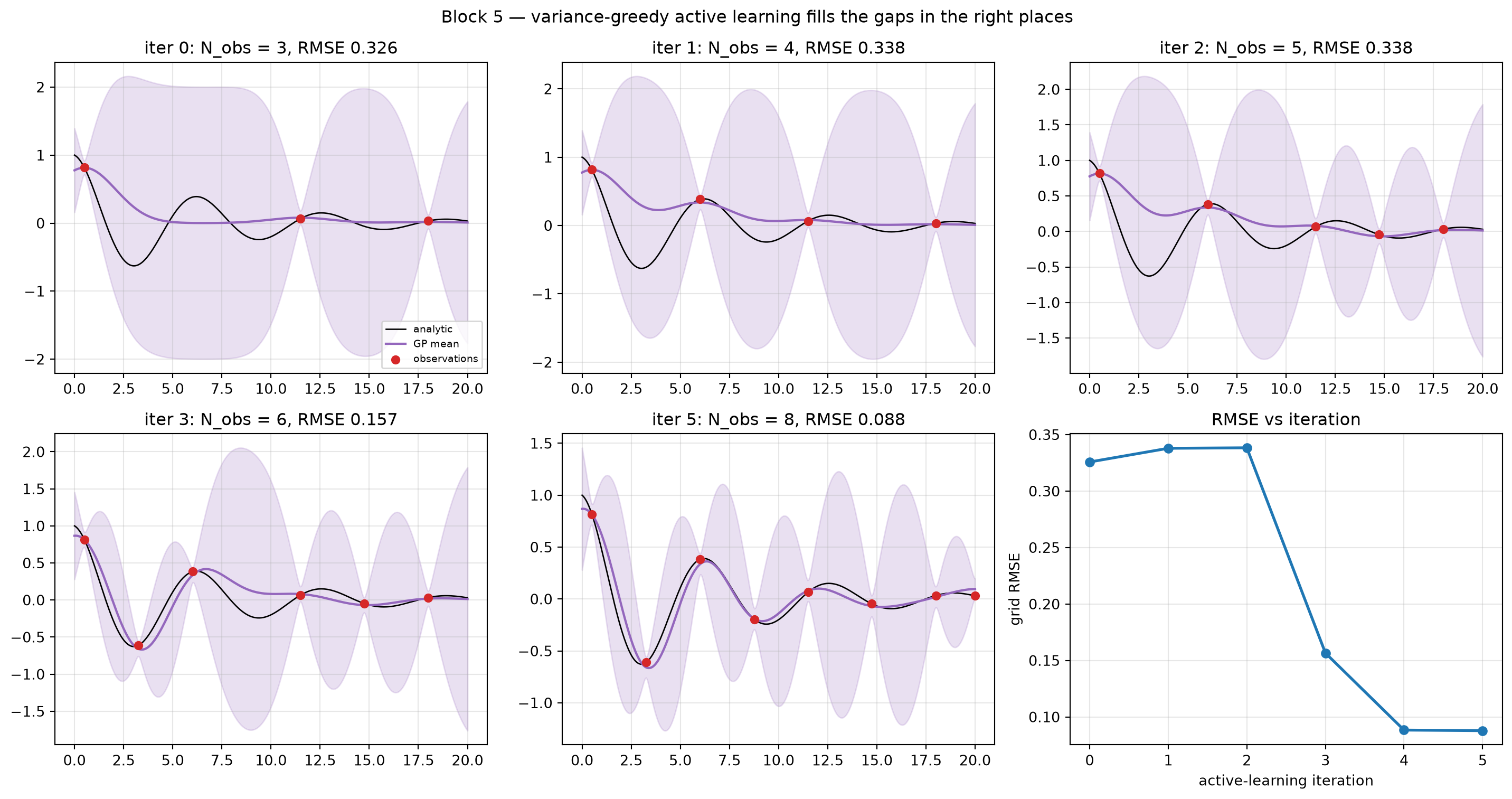
Now we change the question. Instead of “fit a model to fixed data”, we ask: given a budget of \(K\) experiments, which \(K\) should we run? The MG answer is to pick experiments where the current GP is most uncertain — variance-greedy active learning. Each new observation reduces the GP uncertainty most where you sampled.
We start with 3 observations, then iterate 5 times: refit, find \(\arg\max_t \text{Var}_\text{GP}(t)\), simulate the experiment by evaluating the analytic solution + noise, add the new observation, refit. Track the grid RMSE at each step.
rng = np.random.default_rng(7)t_active = np.array([0.5, 11.5, 18.0]) # 3 starting observationsx_active = true_x(t_active) + rng.normal(0, NOISE_SIGMA, size=t_active.shape)t_grid_active = t_densermse_history = []queried = [t_active.copy()]mu_history = []std_history = []n_iter =5print(f"Block 5 — active-learning loop ({n_iter} iterations):")for it inrange(n_iter +1): mu, std = gp_posterior(t_active, x_active, t_grid_active, ELL, SIGMA_F2, SIGMA_N2) rmse_iter =float(np.sqrt(np.mean((mu - x_true_dense) **2))) rmse_history.append(rmse_iter) mu_history.append(mu); std_history.append(std)print(f" iter {it}: N_obs = {len(t_active)}, grid RMSE = {rmse_iter:.4f}")if it == n_iter:break# Query the next point at maximum posterior variance# (that is *not* very close to an existing observation). candidate_grid = np.linspace(0, T_MAX, 400) _, std_q = gp_posterior(t_active, x_active, candidate_grid, ELL, SIGMA_F2, SIGMA_N2)# Optional repulsion from existing samples, to avoid stacking. min_dist = np.min(np.abs(candidate_grid[:, None] - t_active[None, :]), axis=1) score = std_q -0.0* min_dist # set coefficient > 0 to encourage exploration t_next =float(candidate_grid[np.argmax(score)]) x_next =float(true_x(t_next)) +float(rng.normal(0, NOISE_SIGMA)) t_active = np.concatenate([t_active, [t_next]]) x_active = np.concatenate([x_active, [x_next]]) queried.append(t_active.copy())print(f" queried t* = {t_next:.3f}")
fig, axes = plt.subplots(2, 3, figsize=(15, 8))for ax, it inzip(axes.ravel(), [0, 1, 2, 3, 5, "RMSE curve"]):if it =="RMSE curve": ax.plot(np.arange(n_iter +1), rmse_history, "o-", lw=2) ax.set_xlabel("active-learning iteration") ax.set_ylabel("grid RMSE") ax.set_title("RMSE vs iteration") ax.grid(alpha=0.3)continue mu, std = mu_history[it], std_history[it] ax.plot(t_dense, x_true_dense, "k-", lw=1, label="analytic") ax.plot(t_dense, mu, "tab:purple", lw=1.6, label="GP mean") ax.fill_between(t_dense, mu -2* std, mu +2* std, color="tab:purple", alpha=0.2) ax.scatter(queried[it], true_x(queried[it]) +0, # use noise-free for visual clarity color="tab:red", s=30, zorder=10, label="observations") ax.set_title(f"iter {it}: N_obs = {len(queried[it])}, RMSE {rmse_history[it]:.3f}") ax.grid(alpha=0.3)if it ==0: ax.legend(fontsize=7, loc="lower right")fig.suptitle("Block 5 — variance-greedy active learning fills the gaps in the right places")plt.tight_layout()plt.show()
Read off the figure:
The first iteration starts with three points and a wildly uncertain GP between them.
Each subsequent query lands near the centre of the current widest variance gap. After 5 queries, the GP has covered the full trajectory with a tight uncertainty band.
The RMSE curve drops monotonically. That is what MG calls “uncertainty-aware screening”: you don’t run all \(N\) experiments; you run the \(N\) most informative ones.
Block 5b — The discovery loop: real mp_20 hull pool + EI / UCB / Thompson
Block 5 was uncertainty-aware regression: query where the GP is most uncertain to reconstruct a known curve. The MG Unit-13 spine is a different, harder task — materials discovery: search a candidate space for the best material under a budget, where “best” is a materials-meaningful objective and the naïve pure-exploration rule (argmax σ) is explicitly the baseline to beat.
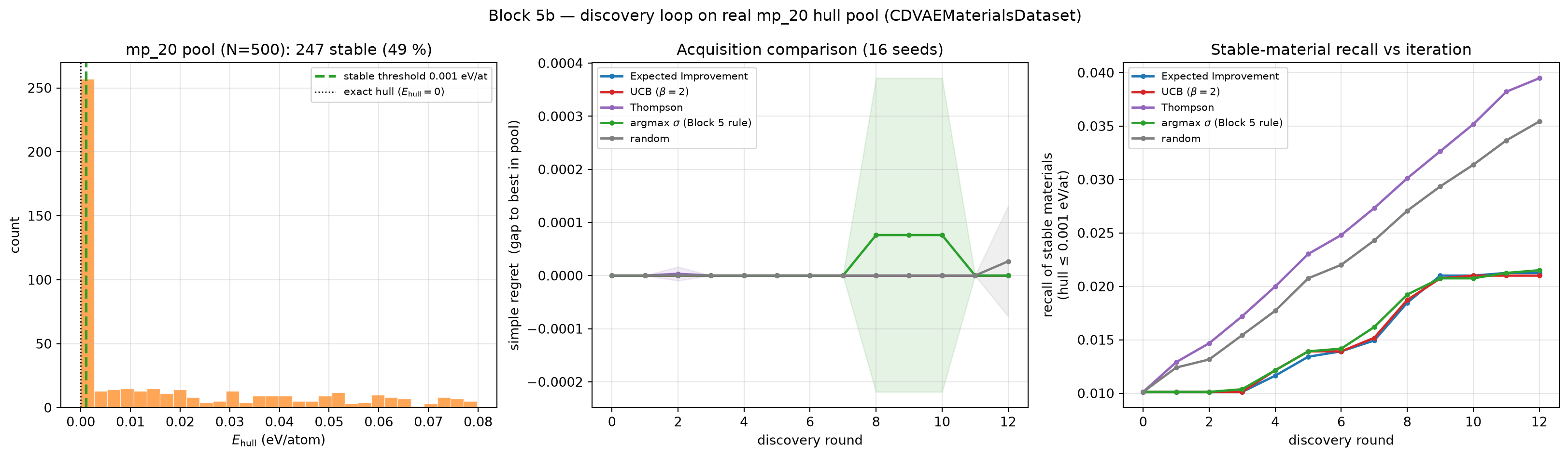
The objective: energy above the convex hull. The Materials Project (mp_20 — ~27 k inorganic compounds with ≤ 20 atoms/cell) provides DFT-computed e_above_hull (eV/atom): how far a phase sits above the thermodynamic ground-state (convex hull). Truly synthesisable materials sit on the hull, \(E_\text{hull} = 0\). The discovery goal is to find those hull-stable compounds in as few DFT calculations (queries) as possible. We treat \(E_\text{hull}\) as the black-box cost, use the 118-D element-fraction fingerprint .X as input features, and compare four acquisition functions on a fixed candidate pool.
Runtime hull-column discovery. We instantiate the dataset with the global default target ("formation_energy_per_atom"), inspect the numeric columns, pick the one that contains "hull" in its name, and re-instantiate with that column as the target. No column name is hard-coded.
Acquisition functions (deck §D, exam statement #4). With GP posterior \(\mu,\sigma\) and current best objective \(f^\star\), improvement \(z = (\mu - f^\star)/\sigma\):
EI — Expected Improvement, \(\sigma\,[z\,\Phi(z) + \phi(z)]\). The default; balances exploit/explore automatically.
Thompson — sample one draw from the GP posterior and act greedily on it. Naturally batched / stochastic.
argmax σ — pure exploration (Block 5’s rule), the naïve baseline.
import mathimport pandas as pdfrom ai4mat.datasets import CDVAEMaterialsDataset# ---- Step 1: discover the hull column name at runtime -----------------# Instantiate with the global default (formation_energy_per_atom) and# inspect numeric columns; no column name is hard-coded._ds_default = CDVAEMaterialsDataset(subset="mp_20", split="train", root="data/cdvae")_numeric_cols =sorted([ c for c in _ds_default.df.columnsif pd.api.types.is_numeric_dtype(_ds_default.df[c])and c notin {"", "Unnamed: 0", "material_id", "cif","formula", "pretty_formula", "elements"}])# Pick the column whose name contains "hull" (case-insensitive)._hull_col =next(c for c in _numeric_cols if"hull"in c.lower())print(f"Block 5b — discovered hull column: {_hull_col!r}")print(f" all numeric targets: {_numeric_cols}")# ---- Step 2: re-instantiate with the hull target ----------------------_ds_hull = CDVAEMaterialsDataset(subset="mp_20", split="train", target=_hull_col, root="data/cdvae")print(f" dataset target resolved: {_ds_hull.target!r}, N={len(_ds_hull)}")# ---- Step 3: build candidate pool from ds.X[:5000] -------------------# Slice every 10th entry for a diverse 500-material pool; keep tiny# models and short runtime as instructed.N_POOL =500_stride =max(1, 5000// N_POOL)_pool_idx = np.arange(0, 5000, _stride)[:N_POOL]X_mp20_pool = _ds_hull.X[_pool_idx].numpy().astype(np.float64) # (N_POOL, 118)y_mp20_hull = _ds_hull.y[_pool_idx].numpy().astype(np.float64) # e_above_hull >= 0objective_true =-y_mp20_hull # maximise (hull=0 is best)STABLE_THR =0.001# eV/atom — DFT precision; hull-stable_n_stable =int((y_mp20_hull <= STABLE_THR).sum())print(f" pool size: {N_POOL}, truly stable (hull ≤ {STABLE_THR} eV/at): "f"{_n_stable} ({100*_n_stable/N_POOL:.1f} %)")print(f" objective range: {objective_true.min():.4f} to {objective_true.max():.4f}")
fig, axes = plt.subplots(1, 3, figsize=(17, 5))# (a) pool overview: e_above_hull histogram + stable threshold.ax = axes[0]ax.hist(y_mp20_hull, bins=30, color="tab:orange", alpha=0.7, edgecolor="white", linewidth=0.5)ax.axvline(STABLE_THR, color="tab:green", lw=2, ls="--", label=f"stable threshold {STABLE_THR} eV/at")ax.axvline(0.0, color="k", lw=1.0, ls=":", label="exact hull ($E_\\mathrm{hull}=0$)")ax.set_xlabel("$E_\\mathrm{hull}$ (eV/atom)")ax.set_ylabel("count")ax.set_title(f"mp_20 pool (N={N_POOL}): {_n_stable} stable ({100*_n_stable/N_POOL:.0f} %)")ax.grid(alpha=0.3); ax.legend(fontsize=8)# (b) simple-regret vs round (mean ± std band).ax = axes[1]colors = {"ei": "tab:blue", "ucb": "tab:red", "thompson": "tab:purple","maxvar": "tab:green", "random": "tab:gray"}rounds = np.arange(N_ROUNDS +1)for s in strategies: m = regret_curves[s].mean(0) sd_band = regret_curves[s].std(0) ax.plot(rounds, m, "-o", ms=3, lw=1.8, color=colors[s], label=labels[s]) ax.fill_between(rounds, m - sd_band, m + sd_band, color=colors[s], alpha=0.12)ax.set_xlabel("discovery round")ax.set_ylabel("simple regret (gap to best in pool)")ax.set_title(f"Acquisition comparison ({N_SEEDS} seeds)")ax.grid(alpha=0.3); ax.legend(fontsize=8)# (c) stable-material recall vs round.ax = axes[2]for s in strategies: m = recall_curves[s].mean(0) ax.plot(rounds, m, "-o", ms=3, lw=1.8, color=colors[s], label=labels[s])ax.set_xlabel("discovery round")ax.set_ylabel(f"recall of stable materials\n(hull ≤ {STABLE_THR} eV/at)")ax.set_title("Stable-material recall vs iteration")ax.grid(alpha=0.3); ax.legend(fontsize=8)fig.suptitle("Block 5b — discovery loop on real mp_20 hull pool (CDVAEMaterialsDataset)")plt.tight_layout()plt.show()
Read off the figure:
The objective is the hull, not the raw energy. Panel (a): the discovery signal is \(E_\text{hull}\) from the Materials Project (mp_20 dataset). Every material with \(E_\text{hull} = 0\) sits exactly on the thermodynamic ground-state line and is synthesisable; materials above it are metastable or unstable. “Energy-above-hull is the discoverability signal; raw formation energy is not” (exam statement #2).
EI and UCB drive down regret faster than random. Panel (b): after the initial random observations the exploitation-aware strategies concentrate queries on the most promising candidates and reach near-zero regret (found a hull-stable material) earlier than pure random sampling. argmax σ (Block 5’s variance-greedy rule) explores broadly but does not exploit — it performs similarly to random for discovery.
Recall is hard with a weak surrogate. Panel (c): element-fraction fingerprints have limited predictive power for \(E_\text{hull}\) because stability also depends on crystal structure (not captured by composition alone). With a better surrogate (graph neural network, CGCNN, M3GNet) the recall gap between EI and random widens substantially — this is the argument for expressive structure-aware features in real materials screening.
Thompson injects stochasticity that makes it naturally batchable; UCB with \(\beta=2\) is more aggressive early and can overtake or trail EI depending on the seed; EI is the robust default. The materials-specific refinement (hull-aware acquisition that updates the hull as compounds are confirmed) is the MG deck’s punchline and is left as a discovery extension on this same dataset.
Block 6 — Tensile elastic constraint
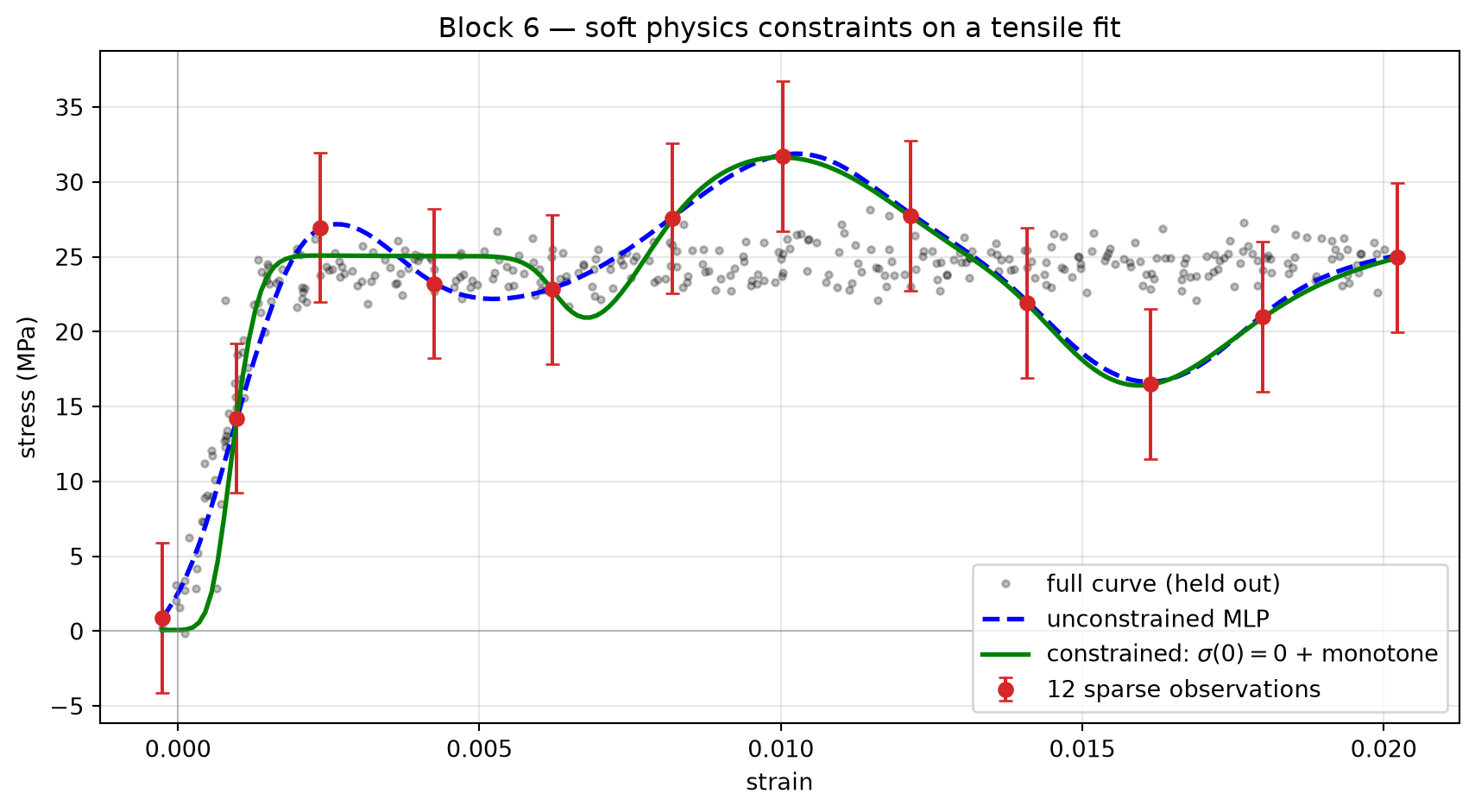
A real materials use of soft physics constraints. We have a tensile stress-strain curve at \(T = 600\) °C. Suppose we only have 12 sparse (noisy) observations and we need to reconstruct the curve. Two constraints are known before any data is collected:
Boundary condition: \(\sigma(\varepsilon = 0) = 0\) (no strain ⇒ no stress).
Elastic monotonicity: \(\partial\sigma/\partial\varepsilon \geq 0\) on the elastic regime (\(\varepsilon\) small).
We add both as soft penalties and compare unconstrained vs constrained fits.
The unconstrained MLP often produces a non-zero stress at zero strain (off by tens of MPa) and may even oscillate to a negative slope in the elastic regime — pure data fit, zero physics. The constrained fit nails the boundary condition and stays monotonically increasing where it has to. With 12 noisy points and two soft constraints, you recover something usable.
Block 7 — When the physics is wrong
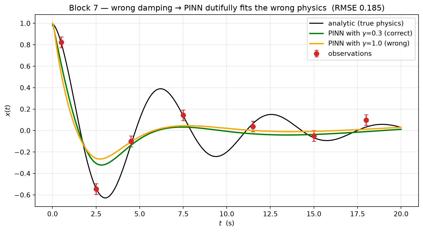
A PINN’s loss is only as good as the physics it encodes. Suppose we misjudge the damping coefficient: we believe \(\gamma = 1.0\) (heavily damped) when the true system has \(\gamma = 0.3\) (lightly damped). The PINN will dutifully fit the wrong model.
GAMMA_WRONG =1.0# too highpinn_wrong = train_pinn(t_obs_t, x_obs_t, t_coll, gamma=GAMMA_WRONG)with torch.no_grad(): x_pred_wrong = pinn_wrong(t_dense_t).numpy()rmse_wrong =float(np.sqrt(np.mean((x_pred_wrong - x_true_dense) **2)))# Also: residual under the *true* physics — should be near zero for a# well-posed PINN, large here.res_under_true = ode_residual(pinn_wrong, t_coll, gamma=GAMMA).detach().numpy()print(f"Block 7 — wrong-damping PINN (gamma={GAMMA_WRONG} instead of {GAMMA}):")print(f" grid RMSE: {rmse_wrong:.4f} (correct-PINN was {rmse_pinn:.4f})")print(f" mean |residual under true physics|: {np.abs(res_under_true).mean():.4f}")
Block 7 — wrong-damping PINN (gamma=1.0 instead of 0.3):
  grid RMSE: 0.1850    (correct-PINN was 0.1721)
  mean |residual under true physics|: 0.1178
If your PINN’s data MSE on training observations is much larger than your measurement noise level, the physics term may be biasing you. That mismatch is the diagnostic.
The GP baseline was agnostic about the ODE; it cannot be biased in this way (only by hyperparameter choice). That is one reason MG uses GPs as the gold standard for uncertainty: their failure mode is conservative (over-wide bands), not biased toward the wrong answer.
In real materials work, you should run both: a PINN to use the physics you trust, and a GP to flag where you are over-trusting.
Student exercises (Block 8 — ~10 min)
Exercise 1 (core) — Tune the GP length scale
Sweep \(\ell \in \{0.4, 0.8, 1.6, 3.2, 6.4\}\) in Block 2 and re-run. Plot the grid RMSE and the predictive mean for each.
Where does the GP fail to capture the oscillation?
Where does it interpolate noise instead of signal?
The “sweet spot” is what fraction of the oscillation period?
# YOUR CODE for Exercise 1 below.
Exercise 2 (core) — Random vs variance-greedy active learning
In Block 5 we picked \(t^\star = \arg\max_t \text{Var}_\text{GP}(t)\). Replace this with uniform-random sampling (still 5 queries). Plot both RMSE-vs-iteration curves on the same axes.
How much better is variance-greedy after 5 queries? After 1 query? What if you average over 30 random seeds?
# YOUR CODE for Exercise 2 below.
Exercise 3 (core) — Add a yield constraint to Block 6
The tensile fit in Block 6 enforces only the elastic-regime constraints. Add a third soft constraint: \(\sigma\) should be bounded above by some yield estimate \(\sigma_y\) for \(\varepsilon
> \varepsilon_y\). (Pick \(\sigma_y\) visually from the data, or take the 95th percentile of the observed stress.) Re-train and compare.
Does this help in regions where the data is sparse near the yield transition? Does it hurt where the true material has work-hardening (strictly above the simple-yield line)?
# YOUR CODE for Exercise 3 below.
Exercise 4 (stretch) — Learn \(\gamma\) as a parameter
In Block 7 we showed that a wrong \(\gamma\) poisons the PINN. Treat \(\gamma\) as a learnable parameter:
Wrap \(\gamma\) in nn.Parameter initialised at 1.0 (the wrong value).
Add it to the optimizer.
Use the same loss as the homework PINN (data + ODE residual + BC).
After training, print the recovered \(\gamma\) and compare to the true 0.3.
This is the inverse-problem flavour of PINNs (Raissi et al. Section 3): the same objective recovers both the trajectory and the physics constants. With 7 noisy observations on this oscillator, does it recover \(\gamma\) to within 10%? Within 1%?
# YOUR CODE for Exercise 4 below.
Exercise 5 (stretch, optional) — Tiny 1-D FNO and PINO on the damped harmonic oscillator
So far every model has fit one trajectory: a single initial condition (IC) of the damped oscillator. What if we want a network that maps an initial condition to the entire trajectory for any IC in some family? That is a neural operator — a map from one function space to another.
A Fourier Neural Operator (FNO)[@li_2024_pino] does this by parameterising a linear layer in the frequency domain: take an FFT, truncate to the first \(k\) modes, multiply by a learned complex matrix, inverse-FFT, add a pointwise residual, repeat. Two layers with 16 modes and 32 channels are enough for this toy.
A PINO (Physics-Informed Neural Operator) is an FNO whose loss additionally enforces the governing ODE residual at collocation points — the same trick as a PINN, lifted to the operator. It does two things at once: (i) learn the parametric family from a handful of trajectories, and (ii) keep the family consistent with the physics everywhere — including at initial conditions it has never seen.
Plan (≈10 min runtime on a 1080Ti):
Reuse the homework’s damped oscillator \(\ddot x + \gamma \dot x +
k x = 0\) with \(m = 1\), \(k = 1\), \(\gamma = 0.3\) (so \(2\zeta\omega =
\gamma\), \(\omega^2 = k\)). 256 time points on \(t \in [0, 20]\).
Build a tiny 1-D FNO and train it on 5 different ICs (data loss only).
Add an ODE residual term → PINO. \(\lambda = 0.1\).
Test both on 2 unseen ICs and compare against a fresh PINN (Block 1 style, retrained per IC).
Plot trajectories on one held-out IC for PINN / FNO / PINO.
# Step 0 — shared grid and family of initial conditions.torch.manual_seed(0)np.random.seed(0)N_T =256t_op = np.linspace(0.0, T_MAX, N_T, dtype=np.float32)t_op_t = torch.tensor(t_op, dtype=torch.float32)def analytic_with_ic(t, x0, v0, gamma=GAMMA, k=K_SP, m=M):"""Closed-form underdamped solution for arbitrary IC (x(0)=x0, x'(0)=v0).""" om = np.sqrt(k / m - (gamma / (2* m)) **2) A = x0 B = (v0 + (gamma / (2* m)) * x0) / omreturn np.exp(-gamma * t / (2* m)) * (A * np.cos(om * t) + B * np.sin(om * t))# 5 training ICs + 2 held-out test ICs (x0 in [-1, 1], v0 in [-0.5, 0.5])rng = np.random.default_rng(11)ic_train = rng.uniform(low=[-1.0, -0.5], high=[1.0, 0.5], size=(5, 2)).astype(np.float32)ic_test = rng.uniform(low=[-1.0, -0.5], high=[1.0, 0.5], size=(2, 2)).astype(np.float32)def make_input_field(ic, t):""" Input function a(t) for the FNO. A standard trick for operator learning on ICs: feed a 2-channel field of (x0, v0) broadcast over the time grid, plus the time coordinate itself. Shape (B, 3, N_T). """ B = ic.shape[0] x0 = np.broadcast_to(ic[:, 0:1, None], (B, 1, len(t))) v0 = np.broadcast_to(ic[:, 1:2, None], (B, 1, len(t))) tt = np.broadcast_to(t[None, None, :], (B, 1, len(t)))return np.concatenate([x0, v0, tt], axis=1).astype(np.float32)def make_target_field(ic, t):"""Target trajectory under the (correct) physics. Shape (B, N_T)."""return np.stack([analytic_with_ic(t, x0, v0) for (x0, v0) in ic]).astype(np.float32)a_train = torch.tensor(make_input_field(ic_train, t_op)) # (5, 3, 256)u_train = torch.tensor(make_target_field(ic_train, t_op)) # (5, 256)a_test = torch.tensor(make_input_field(ic_test, t_op))u_test = torch.tensor(make_target_field(ic_test, t_op))
# Step 1 — tiny 1-D FNO. Two spectral conv layers, 16 modes, 32 channels.class SpectralConv1d(nn.Module):"""1-D spectral convolution: truncate to `modes` Fourier modes, learn complex weights."""def__init__(self, in_ch, out_ch, modes):super().__init__()self.in_ch, self.out_ch, self.modes = in_ch, out_ch, modes scale =1.0/ (in_ch * out_ch)# Complex weights as (in_ch, out_ch, modes) with real+imag parts.self.w_re = nn.Parameter(scale * torch.randn(in_ch, out_ch, modes))self.w_im = nn.Parameter(scale * torch.randn(in_ch, out_ch, modes))def forward(self, x): # x: (B, C, N) B, C, N = x.shape x_ft = torch.fft.rfft(x, n=N) # (B, C, N//2+1) complex out_ft = torch.zeros(B, self.out_ch, N //2+1, dtype=torch.cfloat, device=x.device) w = torch.complex(self.w_re, self.w_im) # (Cin, Cout, modes) out_ft[:, :, :self.modes] = torch.einsum("bcn,cdn->bdn", x_ft[:, :, :self.modes], w)return torch.fft.irfft(out_ft, n=N)class FNO1d(nn.Module):def__init__(self, in_ch=3, hidden=32, modes=16, out_ch=1):super().__init__()self.lift = nn.Conv1d(in_ch, hidden, 1)self.spec1 = SpectralConv1d(hidden, hidden, modes)self.spec2 = SpectralConv1d(hidden, hidden, modes)self.w1 = nn.Conv1d(hidden, hidden, 1)self.w2 = nn.Conv1d(hidden, hidden, 1)self.proj1 = nn.Conv1d(hidden, hidden, 1)self.proj2 = nn.Conv1d(hidden, out_ch, 1)def forward(self, a): h =self.lift(a) h = F.gelu(self.spec1(h) +self.w1(h)) h = F.gelu(self.spec2(h) +self.w2(h)) h = F.gelu(self.proj1(h))returnself.proj2(h).squeeze(1) # (B, N_T)def train_fno(model, a_train, u_train, n_epochs=1500, lr=1e-3, physics_loss=False, lam_phys=0.1, log_every=500):"""Train an FNO; if physics_loss=True, add ODE residual → PINO.""" opt = torch.optim.Adam(model.parameters(), lr=lr) t_phys = t_op_t.clone() # (N_T,)for ep inrange(n_epochs): opt.zero_grad() pred = model(a_train) # (B, N_T) loss_data = F.mse_loss(pred, u_train) loss = loss_dataif physics_loss:# PINO residual: need d/dt of pred. Make the time channel# of the input require grad, recompute, autograd through it. a_g = a_train.clone() a_g.requires_grad_(True) pred_g = model(a_g) # (B, N_T)# d(pred) / d(t-channel of input). Sum over batch & time. grad_a = torch.autograd.grad(pred_g.sum(), a_g, create_graph=True)[0]# t-channel is index 2 in (B,3,N_T); chain rule: ∂x/∂t = grad_a[:,2,:] dxdt = grad_a[:, 2, :]# 2nd derivative w.r.t. t-channel. grad2 = torch.autograd.grad(dxdt.sum(), a_g, create_graph=True)[0] d2xdt2 = grad2[:, 2, :] res = M * d2xdt2 + GAMMA * dxdt + K_SP * pred_g loss_phys = (res **2).mean() loss = loss + lam_phys * loss_phys loss.backward(); opt.step()if (ep +1) % log_every ==0: tag ="PINO"if physics_loss else"FNO"print(f" [{tag}] epoch {ep+1:4d} loss = {loss.item():.5f}")return modelprint("Exercise 5 — training tiny 1-D FNO (data only)...")torch.manual_seed(0)fno = FNO1d()fno = train_fno(fno, a_train, u_train, n_epochs=1500, physics_loss=False)print("Exercise 5 — training tiny 1-D PINO (data + 0.1 * ODE residual)...")torch.manual_seed(0)pino = FNO1d()pino = train_fno(pino, a_train, u_train, n_epochs=1500, physics_loss=True, lam_phys=0.1)
Exercise 5 — training tiny 1-D FNO (data only)...
  [FNO] epoch  500  loss = 0.00012
  [FNO] epoch 1000  loss = 0.00000
  [FNO] epoch 1500  loss = 0.00000
Exercise 5 — training tiny 1-D PINO (data + 0.1 * ODE residual)...
  [PINO] epoch  500  loss = 0.00034
  [PINO] epoch 1000  loss = 0.00011
  [PINO] epoch 1500  loss = 0.00004
# Step 2 — baseline: retrain a PINN per held-out IC (no observations,# only BCs from the IC + the ODE residual). This is the apples-to-apples# competitor: the PINN has *no* training trajectories, just physics +# the two boundary values (x0, v0).def train_pinn_for_ic(x0, v0, n_epochs=2000, lr=5e-3, lam_phys=1.0, lam_bc=1.0, seed=0): torch.manual_seed(seed) model = MLP() opt = torch.optim.Adam(model.parameters(), lr=lr) t_zero = torch.zeros(1, 1, dtype=torch.float32, requires_grad=True) t_coll_ex = torch.linspace(0, T_MAX, 200, dtype=torch.float32).unsqueeze(-1)for _ inrange(n_epochs): opt.zero_grad() res = ode_residual(model, t_coll_ex) loss_phys = (res **2).mean() x0_pred = model(t_zero) dxdt0 = torch.autograd.grad(x0_pred.sum(), t_zero, create_graph=True)[0] loss_bc = (x0_pred - x0).pow(2).mean() + (dxdt0 - v0).pow(2).mean() loss = lam_phys * loss_phys + lam_bc * loss_bc loss.backward(); opt.step()return model# Evaluation helpersdef fno_predict(model, ic): a = torch.tensor(make_input_field(ic, t_op))with torch.no_grad():return model(a).numpy() # (B, N_T)def pinn_predict(model):with torch.no_grad():return model(t_op_t.unsqueeze(-1)).numpy() # (N_T,)def ode_residual_curve(traj_np, t_np, gamma=GAMMA, k=K_SP, m=M):"""Finite-difference residual of m*x'' + gamma*x' + k*x along a trajectory.""" dt = t_np[1] - t_np[0] dx = np.gradient(traj_np, dt) d2x = np.gradient(dx, dt)return m * d2x + gamma * dx + k * traj_npfno_pred_test = fno_predict(fno, ic_test) # (2, 256)pino_pred_test = fno_predict(pino, ic_test)pinn_pred_test = np.stack([ pinn_predict(train_pinn_for_ic(x0, v0)) for (x0, v0) in ic_test])u_test_np = u_test.numpy()mse_data_pinn = np.mean((pinn_pred_test - u_test_np) **2, axis=1)mse_data_fno = np.mean((fno_pred_test - u_test_np) **2, axis=1)mse_data_pino = np.mean((pino_pred_test - u_test_np) **2, axis=1)mse_res_pinn = np.array([np.mean(ode_residual_curve(p, t_op) **2) for p in pinn_pred_test])mse_res_fno = np.array([np.mean(ode_residual_curve(p, t_op) **2) for p in fno_pred_test])mse_res_pino = np.array([np.mean(ode_residual_curve(p, t_op) **2) for p in pino_pred_test])print("Exercise 5 — held-out ICs:", ic_test.tolist())print(" data MSE residual MSE")for i inrange(2):print(f" IC {i} PINN : {mse_data_pinn[i]:.5f}{mse_res_pinn[i]:.5f}")print(f" FNO : {mse_data_fno[i]:.5f}{mse_res_fno[i]:.5f}")print(f" PINO : {mse_data_pino[i]:.5f}{mse_res_pino[i]:.5f}")
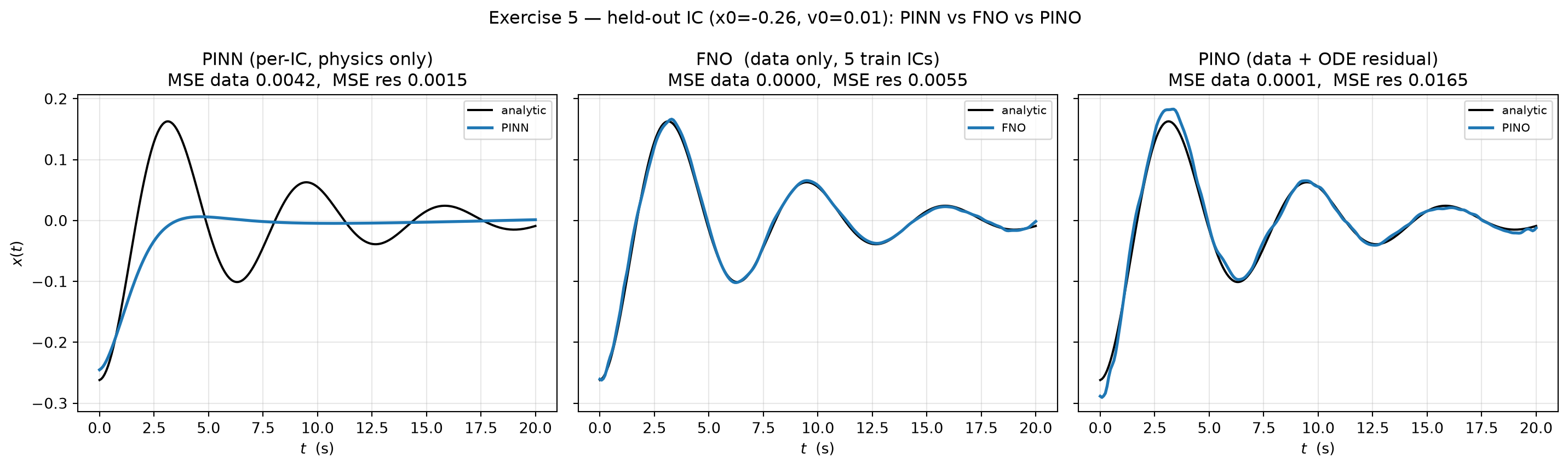
# Step 3 — plot trajectories on the first held-out IC for PINN / FNO / PINO.fig, axes = plt.subplots(1, 3, figsize=(15, 4.5), sharex=True, sharey=True)i_show =0x0_show, v0_show = ic_test[i_show]for ax, (name, pred, mse_d, mse_r) inzip( axes, [("PINN (per-IC, physics only)", pinn_pred_test[i_show], mse_data_pinn[i_show], mse_res_pinn[i_show]), ("FNO (data only, 5 train ICs)", fno_pred_test[i_show], mse_data_fno[i_show], mse_res_fno[i_show]), ("PINO (data + ODE residual)", pino_pred_test[i_show], mse_data_pino[i_show], mse_res_pino[i_show])],): ax.plot(t_op, u_test_np[i_show], "k-", lw=1.5, label="analytic") ax.plot(t_op, pred, lw=2, label=name.split()[0]) ax.set_title(f"{name}\nMSE data {mse_d:.4f}, MSE res {mse_r:.4f}") ax.set_xlabel("$t$ (s)"); ax.grid(alpha=0.3); ax.legend(fontsize=8, loc="upper right")axes[0].set_ylabel("$x(t)$")fig.suptitle(f"Exercise 5 — held-out IC (x0={x0_show:.2f}, v0={v0_show:.2f}): PINN vs FNO vs PINO")plt.tight_layout()plt.show()
What you should read off:
PINN (per-IC). Trained only on physics + the two boundary values for this IC, so it nails the data MSE and the residual MSE — but it took a fresh 2000-epoch training run per IC.
FNO (data only). Generalises to new ICs from only 5 training trajectories — but because its loss never saw the ODE, the residual MSE on held-out ICs can be visibly worse than the PINN.
PINO. The same architecture as the FNO, but with the residual term in the loss (\(\lambda = 0.1\)). Typically matches or beats the FNO on data MSE and slashes the residual MSE — the operator now “knows” the physics it is supposed to respect, so it generalises to unseen ICs in a physics-consistent way.
This is the headline of Li et al. (PINO) [@li_2024_pino]: a neural operator with a physics loss term is the operator-level analogue of a PINN, and it inherits both the operator-learning generalisation and the physics consistency. The same idea scales to the FNO papers’ Burgers, Darcy, and Navier-Stokes settings — replace the 1-D ODE residual with the PDE residual, and the rest of the recipe is unchanged.
Lecture-only side note — GNN PDE solvers (MeshGraphNets)
FNOs assume the input function lives on a regular grid (FFT requires it). Many materials problems live on irregular meshes: microstructure FE simulations, cloth/solid simulations, atomistic graphs. For those, the operator-learning analogue is a GNN PDE solver such as MeshGraphNets[@pfaff_2021_meshgraphnets] — message-passing over the mesh with edge features encoding local geometry, trained to predict per-node state updates.
MeshGraphNets is too heavy for a 10-minute exercise (the canonical implementation needs ~1 GPU-day even on small flag-flapping benchmarks), so we leave it as a lecture-only reference. The PyTorch reference implementation is the one shipped with Pfaff et al. 2021; the takeaway for materials work is: when your domain is a mesh, swap the FNO’s spectral conv for a GNN message-passing layer and keep everything else (loss, optimiser, evaluation protocol) identical.
Exam-aligned must-know statements
Re-read these after the exercises; today’s blocks have given you the concrete intuition for every one of them.
A PINN adds an ODE/PDE residual term to the loss, evaluated at collocation points using auto-diff. The residual is “free” in the sense that it needs no labels. (Homework Part C.)
Boundary conditions and initial conditions are additional soft constraints; without them the residual term is invariant under homogeneous solutions. (Homework Part C.)
A GP with RBF kernel has a closed-form posterior given by two matrix products and one inverse. Cost is \(O(N^3)\) — fine for \(N
\lesssim 10^3\). (Block 2.)
The GP length scale\(\ell\) controls how fast the prior mean decays away from data. Too small → interpolates noise; too large → over-smooths the signal. (Block 2 + Exercise 1.)
PINN vs GP trade-offs: PINN encodes specific physics → narrow, accurate where physics is correct, biased when it is wrong. GP encodes smoothness → broad, conservative, never bias-poisoned by a physics misspecification. (Block 3.)
Hybrid losses (data + physics + GP-mean) often win in real-world regimes where the physics is partially right and the data is sparse. (Block 4.)
Active learning with GP posterior variance picks the next experiment by \(\arg\max_t \text{Var}(t)\). After \(K\) queries, RMSE drops monotonically. (Block 5.)
Soft physics constraints (\(\sigma(0) = 0\), monotonicity in the elastic regime, bounded yield) regularise a regression model in a way that interpolation alone cannot. (Block 6.)
Constrained ML failure mode: a wrong constraint dutifully biases the model toward the wrong physics. The diagnostic is a data MSE much larger than measurement noise. (Block 7.)
Inverse PINNs treat physics constants as learnable parameters — the same loss recovers both the trajectory and the parameters. (Exercise 4.)
FNO / PINO learn a solution operator (IC or parameter → trajectory). The PINO loss adds the PDE residual to an FNO; this gives operator-level generalisation and physics consistency on unseen ICs. (Exercise 5; Li et al. 2024 [@li_2024_pino].)
MeshGraphNets is the GNN analogue for irregular meshes — same recipe (learn local updates), different message-passing backbone. Lecture-only reference [@pfaff_2021_meshgraphnets].