Week 14 — Explainability, limits, and a course retrospective
This is the final Thursday of the SS26 sequence. We braid three lectures’ Week 14 content onto one deployment-audit story:
MFML Unit 14 — Explainability, limits, scientific trust. SHAP, Integrated Gradients, counterfactuals, OOD detection, the six levels of explainability, and a first look at mechanistic interpretability (superposition, sparse autoencoders).
ML-PC Unit 13 — Integration, limits, reflection. Why ML fails in real labs; explainability for experimental ML; instrument drift and distribution shift in practice.
MG Unit 14 — Physical constraints, limits, outlook. Symmetry constraints; what ML can and cannot discover; how the pipeline integrates with experimental workflows.
Red thread.A 95%-accurate model has 5% wrong predictions — the only useful question is which 5%. Today we instrument the tensile regression model from Week 7 with SHAP to learn why each prediction is what it is, train a sparse autoencoder on the Ising-CNN’s hidden activations to ask what concepts the network represents internally (mechanistic interpretability), generate counterfactual explanations for what would have to change to flip a decision, audit the Ising classifier from Week 10 for symmetry equivariance the physics demands, build an autoencoder-based OOD detector that beats the homework’s max-softmax baseline, and end with a retrospective of the 14-week arc — every method on the same problem, with a single chart that says when each one wins.
Pre-flight check. This notebook assumes you have run notebooks/week14_homework.py. Block 1 picks up directly from your trained TinyCNN and your max-softmax-probability OOD scores.
Agenda (90 min)
Block
Min
Topic
1
6
Recap from homework
2
14
KernelSHAP from scratch on a tensile regression model
2b
10
The confounder trap — faithful-to-model ≠ true-of-world
3
12
Sparse autoencoder on Ising-CNN activations — mechanistic interp.
4
14
Counterfactuals via gradient descent on the input
5
12
Symmetry audit on the Ising CNN; fix with test-time augmentation
6
12
Autoencoder reconstruction error as an OOD detector — beats MSP
7
10
Course retrospective: 14 weeks, one chart
8
10
Student exercises (3 core + 1 stretch)
import mathimport numpy as npimport torchimport torch.nn as nnimport torch.nn.functional as Ffrom torch.utils.data import DataLoader, TensorDataset, random_splitimport matplotlib.pyplot as pltfrom sklearn.metrics import roc_auc_scorefrom sklearn.preprocessing import StandardScalerfrom ai4mat.datasets import IsingDataset, CahnHilliardDataset, TensileTestDatasetnp.random.seed(0)torch.manual_seed(0)
<torch._C.Generator at 0x7ff2b0d1a3b0>
Helpers used by every block
class TinyCNN(nn.Module):def__init__(self, n_classes: int=2):super().__init__()# Split into trunk + head so Block 3 can tap the penultimate# 64-dim feature vector (post-pool, pre-classifier).self.trunk = nn.Sequential( nn.Conv2d(1, 16, 3, padding=1), nn.GELU(), nn.Conv2d(16, 32, 3, padding=1), nn.GELU(), nn.Conv2d(32, 64, 3, padding=1), nn.GELU(), nn.AdaptiveAvgPool2d(1), nn.Flatten(), )self.head = nn.Linear(64, n_classes)def features(self, x):"""Penultimate-layer activations (64-dim)."""returnself.trunk(x)def forward(self, x):returnself.head(self.trunk(x))def train_cnn(model, X, y, n_epochs=5, lr=3e-3, batch=128, val_frac=0.1, seed=0): torch.manual_seed(seed) n_val =int(val_frac *len(X)) n_tr =len(X) - n_val ds = TensorDataset(X, y) tr, va = random_split(ds, [n_tr, n_val], generator=torch.Generator().manual_seed(seed)) tr_dl = DataLoader(tr, batch_size=batch, shuffle=True) va_dl = DataLoader(va, batch_size=batch, shuffle=False) opt = torch.optim.AdamW(model.parameters(), lr=lr, weight_decay=1e-4)for ep inrange(n_epochs): model.train()for xb, yb in tr_dl: opt.zero_grad() F.cross_entropy(model(xb), yb).backward() opt.step() model.eval() correct = total =0with torch.no_grad():for xb, yb in va_dl: correct += (model(xb).argmax(-1) == yb).sum().item() total +=len(yb)return correct / total, va
Block 1 — Recap from homework
Three results travel into today:
A small CNN reaches >95% on Ising-light in 5 epochs.
Vanilla saliency (|x · grad|) gives a per-pixel attribution but is biased near saturated activations.
Integrated Gradients fixes this with a baseline-relative line integral and satisfies the completeness axiom: the per-pixel attributions sum to \(f_c(x) - f_c(\text{baseline})\).
Max softmax probability is a cheap OOD baseline; AUROC was moderate vs Cahn-Hilliard, weaker vs shuffled Ising. Block 6 will do better with reconstruction error.
We re-train the CNN here so today’s session is self-contained.
ising = IsingDataset(size="light")cnn = TinyCNN()val_acc, ising_val = train_cnn(cnn, ising.X, ising.y)print(f"Block 1 — TinyCNN re-trained on Ising-light: val acc = {val_acc:.3f}")
Block 1 — TinyCNN re-trained on Ising-light: val acc = 0.954
Block 2 — KernelSHAP from scratch on a tensile regression model
SHAP (Lundberg & Lee 2017) gives a per-feature attribution that satisfies four axioms (efficiency, symmetry, dummy, additivity) and generalises Shapley values from cooperative game theory to ML. The kernel version regresses the model on subsets of “active” vs “background” features, weighted by the Shapley kernel \[
w(|S|) = \frac{n - 1}{\binom{n}{|S|} \cdot |S| \cdot (n - |S|)}.
\]
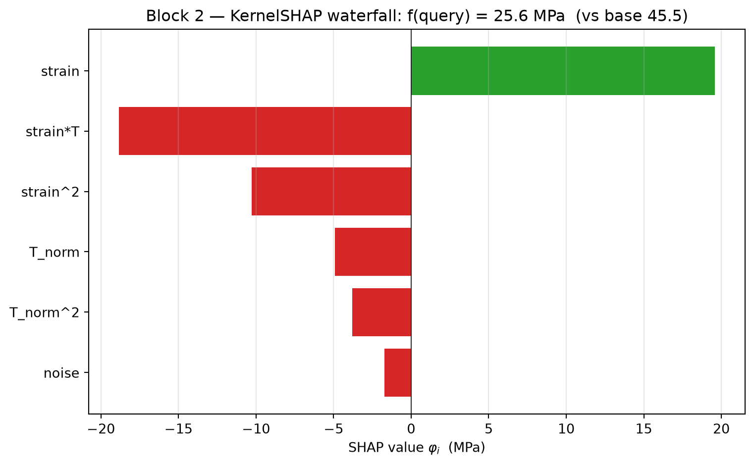
We build a small tensile regression model whose input is enriched: physically meaningful features (strain, \(T\)), engineered cross terms (\(\varepsilon^2\), \(\varepsilon \cdot T\), \(T^2\)), and a pure noise feature. SHAP should attribute high importance to the real features, lower to the engineered ones, and ~0 to the noise.
# Waterfall-style plot.order = np.argsort(np.abs(phi_phys))fig, ax = plt.subplots(figsize=(8, 5))colors = ["tab:red"if p <0else"tab:green"for p in phi_phys[order]]ax.barh(np.array(feat_names)[order], phi_phys[order], color=colors)ax.axvline(0, color="k", lw=0.6)ax.set_xlabel(r"SHAP value $\varphi_i$(MPa)")ax.set_title(f"Block 2 — KernelSHAP waterfall: f(query) = {pred_phys:.1f} MPa (vs base {base_phys:.1f})")ax.grid(alpha=0.3, axis="x")plt.tight_layout()plt.show()
Read the chart:
Real physical features (strain, T_norm, and their squared versions) carry most of the attribution.
The pure noise feature receives ~0 attribution — the model correctly ignores it. This is the SHAP soundness check: features that have no causal link to the target should attribute to ~0.
Sum of \(\varphi_i\) matches \(f(x) - f(\text{background})\) — the efficiency axiom holds (modulo a small numerical correction applied at the end of kernel_shap).
Block 2b — The confounder trap: SHAP is faithful-to-model, not true-of-world
MFML §9 conceptual climax + ML-PC “causality in the process chain” — one block, both lectures.
Block 2’s soundness check rested on a quiet assumption: that a feature with no causal link to the target attributes to ~0. That is only true if the feature is also uncorrelated with the real causes. In a real lab it almost never is. Samples are made in campaigns: a furnace, a powder lot, a measurement session. A furnace_id-style column does not cause strength — yet if hotter campaigns happened to run on furnace B, furnace_id is correlated with \(T\), and a model will happily route prediction through it.
This is the process-chain causality point: composition → processing → microstructure → properties is the causal graph, but the recorded table also carries campaign metadata that is merely correlated with the causal path. A model that maximises accuracy does not know the difference. SHAP, faithfully, will report whatever the model actually used — faithful-to-model is not true-of-world.
Construction (exactly the TODO’s recipe): take the same tensile task and replace the inert noise column with a synthetic furnace_id — the logged processing campaign. The campaign was scheduled by temperature, so furnace_id is a near-deterministic function of \(T\). Crucially, the logged campaign ID is exact, whereas the recorded T_norm carries thermocouple measurement noise (as in a real lab). That gives the model a genuine reason to route the temperature signal through the cleaner confounder — which is exactly how confounders sneak into production models. It is still causally inert: y is generated only by the TensileTestDataset physics, which never sees furnace_id. We then:
train an MLP that reaches good accuracy partly via the confounder,
show SHAP attributes real importance to furnace_id,
run two diagnostics that expose the spurious dependence — permutation importance (predictive, observational) and a controlled intervention (do(furnace_id): resample the confounder independently of \(T\), breaking the back-door path),
read off the correlation-vs-causation moral.
# Build the confounded feature matrix: feature 5 is now `furnace_id`# instead of pure noise, and the recorded `T_norm` (feature 1) is now# a *noisy* thermocouple reading. furnace_id is the exact logged# campaign -> a strong, clean *statistical* proxy for the real driver# T, while being causally inert w.r.t. strength (it never enters the# data-generating physics of `y`).def load_confounded_features():"""Same task as load_tensile_features, but feature 5 = furnace_id. furnace_id encodes the processing campaign. Campaigns were run at a fixed temperature, so furnace_id ~ a noisy bijection of T. It has *no* causal effect on the measured strength `y` (y comes only from the TensileTestDataset physics, which never sees furnace_id). """ rng = np.random.default_rng(1) Xs, ys = [], []# Campaign map: each T was processed on its own furnace. The# logged campaign ID is *exact* (it is metadata, not a sensor). furnace_of_T = {0: 0.0, 400: 1.0, 600: 2.0}for T in [0, 400, 600]: ds = TensileTestDataset(temperature=T) s = ds.X.numpy().reshape(-1) st = ds.y.numpy().reshape(-1) T_true = (T -300.0) /300.0# Recorded T_norm carries thermocouple noise: the *observed*# temperature feature is a noisy reading of the true T that# actually drove the physics in `y`. T_norm = T_true + rng.normal(scale=0.30, size=s.shape)# furnace_id = the exact logged campaign -> a *cleaner* proxy# for the true driver than the noisy thermocouple, so a model# has a real incentive to route temperature through it. fid = np.full_like(s, furnace_of_T[T]) feats = np.stack([s, # strain (causal) T_norm, # T_norm (causal, NOISY) s **2, # strain^2 (causal) s * T_norm, # strain*T (causal) T_norm **2, # T_norm^2 (causal) fid], # furnace_id (CONFOUNDER) axis=1) Xs.append(feats); ys.append(st)return np.concatenate(Xs), np.concatenate(ys), ["strain", "T_norm", "strain^2", "strain*T", "T_norm^2", "furnace_id" ]X_c, y_c, feat_names_c = load_confounded_features()scaler_c = StandardScaler().fit(X_c)X_cs = scaler_c.transform(X_c).astype(np.float32)# Reuse Block 2's target normalisation (same underlying y).y_cs = ((y_c - y_t_mean) / y_t_sd).astype(np.float32)# Confirm the confounding: furnace_id is strongly correlated with T,# but causally inert w.r.t. y by construction.corr_fid_T = np.corrcoef(X_c[:, 5], X_c[:, 1])[0, 1]print(f"Block 2b — corr(furnace_id, T_norm) = {corr_fid_T:+.3f} "f"(strong statistical proxy for the real driver)")
Block 2b — corr(furnace_id, T_norm) = +0.922 (strong statistical proxy for the real driver)
# Train a fresh MLP on the confounded matrix. It is free to use# furnace_id; nothing stops it, and the correlation makes it useful.X_cs_t = torch.tensor(X_cs)y_cs_t = torch.tensor(y_cs)torch.manual_seed(0)mlp_c = TensileMLP()opt_c = torch.optim.AdamW(mlp_c.parameters(), lr=3e-3, weight_decay=1e-4)for _ inrange(800): opt_c.zero_grad() F.mse_loss(mlp_c(X_cs_t), y_cs_t).backward() opt_c.step()mlp_c.eval()with torch.no_grad(): r2_c =1.0- (F.mse_loss(mlp_c(X_cs_t), y_cs_t).item()/ y_cs_t.var(unbiased=False).item())print(f"Block 2b — confounded MLP fit: R^2 = {r2_c:.3f} "f"(good accuracy — but partly via the confounder, shown next)")def mlp_c_predict_np(X_np: np.ndarray) -> np.ndarray:with torch.no_grad():return mlp_c(torch.tensor(X_np, dtype=torch.float32)).numpy()
Block 2b — confounded MLP fit: R^2 = 0.986 (good accuracy — but partly via the confounder, shown next)
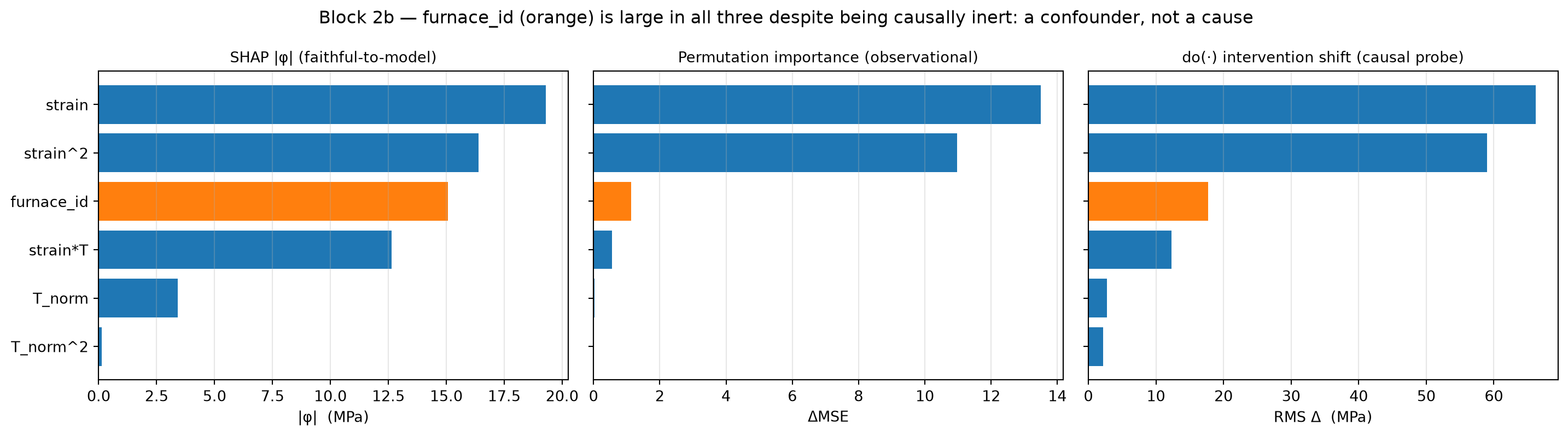
# Diagnostic 1 — SHAP. Faithful-to-model: it will report furnace_id# importance because the model genuinely used it.i_q =int(np.argmax(np.abs(X_cs[:, 0]) + (X_cs[:, 1] >0.8)))x_q = X_cs[i_q]bg_c = X_cs.mean(axis=0)phi_c, base_c, pred_c = kernel_shap(mlp_c_predict_np, x_q, bg_c, n_samples=600)phi_c_phys = phi_c * y_t_sdprint("Block 2b — KernelSHAP on the confounded model "f"(sample {i_q}), per-feature |phi| (MPa):")for n, p insorted(zip(feat_names_c, phi_c_phys), key=lambda v: -abs(v[1])): flag =" <-- CONFOUNDER, causally inert"if n =="furnace_id"else""print(f" {n:<10}: {p:>+8.2f}{flag}")print(" SHAP is *faithful to the model*: it reports furnace_id because")print(" the model used it -- not because furnace_id causes strength.")
Block 2b — KernelSHAP on the confounded model (sample 1048), per-feature |phi| (MPa):
    strain    :   +19.30
    strain^2  :   -16.40
    furnace_id:   -15.06  <-- CONFOUNDER, causally inert
    strain*T  :   -12.65
    T_norm    :    +3.41
    T_norm^2  :    -0.14
  SHAP is *faithful to the model*: it reports furnace_id because
  the model used it -- not because furnace_id causes strength.
# Diagnostic 2 — permutation importance (observational) vs a# controlled intervention do(furnace_id) (causal probe).## Permutation importance: shuffle one column, measure MSE increase.# Because furnace_id ~ T, shuffling it *destroys the proxy* and the# model loses the accuracy it was borrowing from the confounder -># permutation importance is HIGH. This is the observational view: it# answers "does the model rely on this column?" (yes) but NOT "does# this column cause y?".def permutation_importance(predict_fn, X_np, y_np, seed=0): rng = np.random.default_rng(seed) base =float(np.mean((predict_fn(X_np) - y_np) **2)) imp = np.zeros(X_np.shape[1])for j inrange(X_np.shape[1]): Xp = X_np.copy() Xp[:, j] = Xp[rng.permutation(len(Xp)), j] imp[j] =float(np.mean((predict_fn(Xp) - y_np) **2)) - basereturn impperm_imp = permutation_importance(mlp_c_predict_np, X_cs, y_cs)# Controlled intervention do(furnace_id): instead of permuting (which# also breaks the furnace_id<->T link the *honest* way), we resample# furnace_id from its marginal *independently of T*. This severs the# back-door path T -> furnace_id while keeping every causal feature at# its real value. A model that learned the true physics is invariant# under this intervention; a model leaning on the confounder is not.rng_iv = np.random.default_rng(2)X_do = X_cs.copy()X_do[:, 5] = X_cs[rng_iv.permutation(len(X_cs)), 5] # do(furnace_id) ~ marginal, ⟂ Twith torch.no_grad(): pred_obs = mlp_c_predict_np(X_cs) pred_do = mlp_c_predict_np(X_do)intervention_shift =float(np.mean((pred_do - pred_obs) **2)) * (y_t_sd **2)print("Block 2b — permutation importance (ΔMSE, std units):")for n, v insorted(zip(feat_names_c, perm_imp), key=lambda kv: -kv[1]): flag =" <-- model leans on the confounder"if n =="furnace_id"else""print(f" {n:<10}: {v:>+8.4f}{flag}")print(f"\n do(furnace_id) intervention: mean prediction shift "f"= {math.sqrt(intervention_shift):.2f} MPa (RMS).")print(" A purely causal model would be ~0 here; a non-zero shift is")print(" the spurious dependence made visible by an *intervention*,")print(" not by an observation.")
Block 2b — permutation importance (ΔMSE, std units):
    strain    : +13.4981
    strain^2  : +10.9715
    furnace_id:  +1.1304  <-- model leans on the confounder
    strain*T  :  +0.5631
    T_norm    :  +0.0282
    T_norm^2  :  +0.0178

  do(furnace_id) intervention: mean prediction shift = 17.77 MPa (RMS).
  A purely causal model would be ~0 here; a non-zero shift is
  the spurious dependence made visible by an *intervention*,
  not by an observation.
# One picture: SHAP attribution vs permutation importance vs the# do-intervention probe, per feature. The confounder is the bar that# is large in all three despite being causally inert.fig, axes = plt.subplots(1, 3, figsize=(15, 4.2), sharey=True)order_c = np.argsort(np.abs(phi_c_phys))names_o = np.array(feat_names_c)[order_c]def _bar(ax, vals, title, xlabel): cols = ["tab:orange"if n =="furnace_id"else"tab:blue"for n in names_o] ax.barh(names_o, vals[order_c], color=cols) ax.axvline(0, color="k", lw=0.6) ax.set_title(title, fontsize=10) ax.set_xlabel(xlabel) ax.grid(alpha=0.3, axis="x")_bar(axes[0], np.abs(phi_c_phys), "SHAP |φ| (faithful-to-model)", "|φ| (MPa)")_bar(axes[1], perm_imp, "Permutation importance (observational)", "ΔMSE")# Per-feature do-probe: shift when only that column is intervened on.do_per_feat = np.zeros(len(feat_names_c))for j inrange(len(feat_names_c)): Xj = X_cs.copy() Xj[:, j] = X_cs[rng_iv.permutation(len(X_cs)), j] do_per_feat[j] = math.sqrt(float(np.mean( (mlp_c_predict_np(Xj) - pred_obs) **2))) * y_t_sd_bar(axes[2], do_per_feat, "do(·) intervention shift (causal probe)", "RMS Δ (MPa)")fig.suptitle("Block 2b — furnace_id (orange) is large in all three despite ""being causally inert: a confounder, not a cause")plt.tight_layout()plt.show()
Correlation vs causation in the process chain — the moral.
The confounded model has good accuracy (high \(R^2\)). Accuracy alone certifies nothing about causal validity.
SHAP did its job perfectly and is still misleading about the world: it faithfully reports furnace_id importance because the model genuinely used it. Faithful-to-model ≠ true-of-world. This is the single highest-probability conceptual exam question in the MFML unit.
Permutation importance confirms the model relies on furnace_id — but it cannot distinguish “relies on a cause” from “relies on a proxy”, because it stays purely observational.
Only the interventiondo(furnace_id) — resampling the confounder independently of \(T\), severing the back-door path — separates prediction from detection / causation. A model that had learned the physics would be invariant under it; the non-zero shift is the spurious dependence made visible.
Process-chain reading. The causal chain is composition → processing → microstructure → properties. furnace_id is campaign metadata riding alongside that chain, correlated with the real driver \(T\) via how experiments were scheduled. Predicting strength from it works until the schedule changes (a new furnace, a re-lotted powder) — then the proxy breaks and the model fails silently. The deployment rule: an attribution to a non-causal feature is a data-collection finding, not a physical one — re-design the sampling or intervene, never trust the proxy.
Fairness footnote (MFML §9 P3). Swap furnace_id for a protected-group proxy and this is exactly the bias-on-a-proxy problem: the model is “accurate” yet routes through a feature it must not use. Same mathematical object, higher stakes.
Block 3 — Sparse autoencoder on Ising-CNN activations
SHAP and Integrated Gradients answer per-prediction questions (“which inputs mattered for this output?”). They are silent on a different question that matters just as much for trust: what concept does a hidden layer of my network represent?
The naive answer — “inspect individual neurons” — fails because neurons are polysemantic: a single hidden unit fires for several unrelated patterns. This is not a bug; it is superposition[@elhage_2022_superposition]. A network with \(d\) neurons can pack many more than \(d\) near-orthogonal features into the same activation space when those features are sparse — the cost is that each neuron becomes a sum over multiple features.
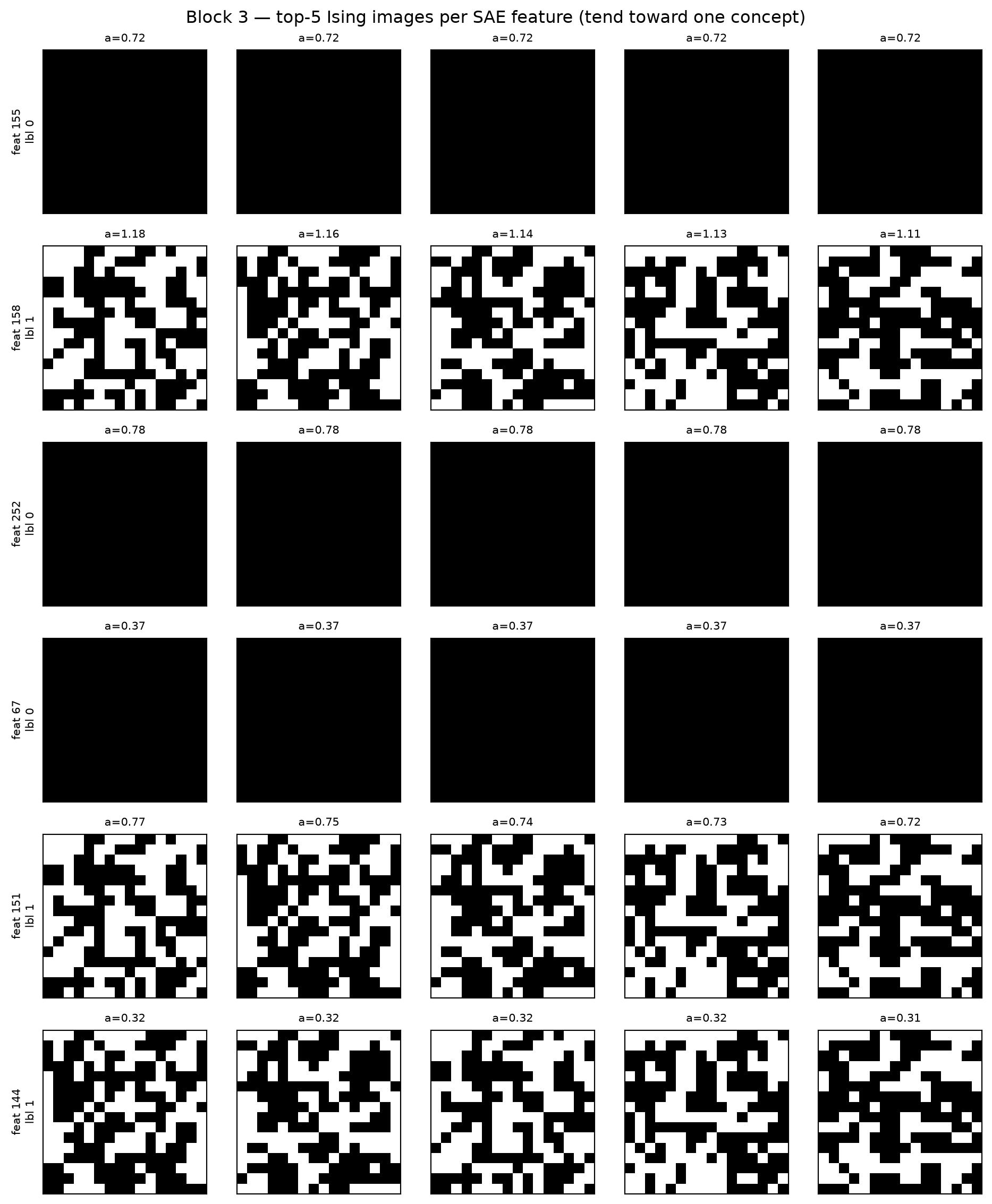
The fix is a wide, sparse autoencoder (SAE) trained on the layer’s activations [@templeton_2024_scaling]. The encoder projects into a higher-dimensional space (\(d' \gg d\)) with an \(\ell_1\) penalty on the post-ReLU code, which forces each input activation to be reconstructed from a small subset of SAE features. The top-activating inputs per SAE feature then tend toward monosemantic concepts — one feature, one idea.
This is exactly the Unit-5 autoencoder with an \(\ell_1\) activation penalty: same encoder/decoder skeleton, same reconstruction loss, one extra term. We apply it to the penultimate (64-dim) layer of the Ising CNN trained in Block 1.
class SparseAutoencoder(nn.Module):"""Wide, sparse autoencoder for mechanistic interpretability. Encoder lifts d -> d' = 4d with ReLU; decoder maps d' -> d. Loss = ||h - h_hat||^2 + lam * ||f||_1, where f is the post-ReLU encoder code. The L1 penalty on the *activations* (not the weights) is what drives monosemanticity. """def__init__(self, d: int, expansion: int=4):super().__init__() d_prime = expansion * dself.enc = nn.Linear(d, d_prime)self.dec = nn.Linear(d_prime, d, bias=False)# A small input bias subtracted before encoding helps centre# activations (cf. Anthropic 2023 SAE recipe).self.b_pre = nn.Parameter(torch.zeros(d))def encode(self, h):return F.relu(self.enc(h -self.b_pre))def forward(self, h): f =self.encode(h) h_hat =self.dec(f) +self.b_prereturn h_hat, ftorch.manual_seed(0)sae = SparseAutoencoder(d=d_act, expansion=4)opt_sae = torch.optim.Adam(sae.parameters(), lr=1e-3)LAM =5e-3N_EPOCHS_SAE =15BATCH_SAE =256print(f"Block 3 — training SAE (d={d_act} -> d'={4*d_act}) for {N_EPOCHS_SAE} epochs, lambda = {LAM}")for ep inrange(N_EPOCHS_SAE): perm = torch.randperm(len(H)) ep_recon = ep_l1 =0.0; n =0for i inrange(0, len(H), BATCH_SAE): hb = H[perm[i : i + BATCH_SAE]] opt_sae.zero_grad() h_hat, f = sae(hb) recon = F.mse_loss(h_hat, hb) l1 = f.abs().mean() loss = recon + LAM * l1 loss.backward(); opt_sae.step() ep_recon += recon.item() *len(hb); ep_l1 += l1.item() *len(hb); n +=len(hb)if ep ==0or (ep +1) %5==0or ep == N_EPOCHS_SAE -1:print(f" epoch {ep+1:>2}: recon MSE {ep_recon/n:.4f} mean |f| {ep_l1/n:.4f}")# Activation frequency per SAE feature.with torch.no_grad(): F_all = sae.encode(H) # (N, d')active = (F_all >0).float().mean(0) # firing rate per featureprint(f" SAE features: {F_all.shape[1]} total, {(active >0).sum().item()} ever active, "f"{(active >0.01).sum().item()} active on >1% of inputs")
Block 3 — training SAE (d=64 -> d'=256) for 15 epochs, lambda = 0.005
  epoch  1: recon MSE 0.2935   mean |f| 0.1913
  epoch  5: recon MSE 0.0048   mean |f| 0.2429
  epoch 10: recon MSE 0.0005   mean |f| 0.2350
  epoch 15: recon MSE 0.0003   mean |f| 0.2298
  SAE features: 256 total, 176 ever active, 174 active on >1% of inputs
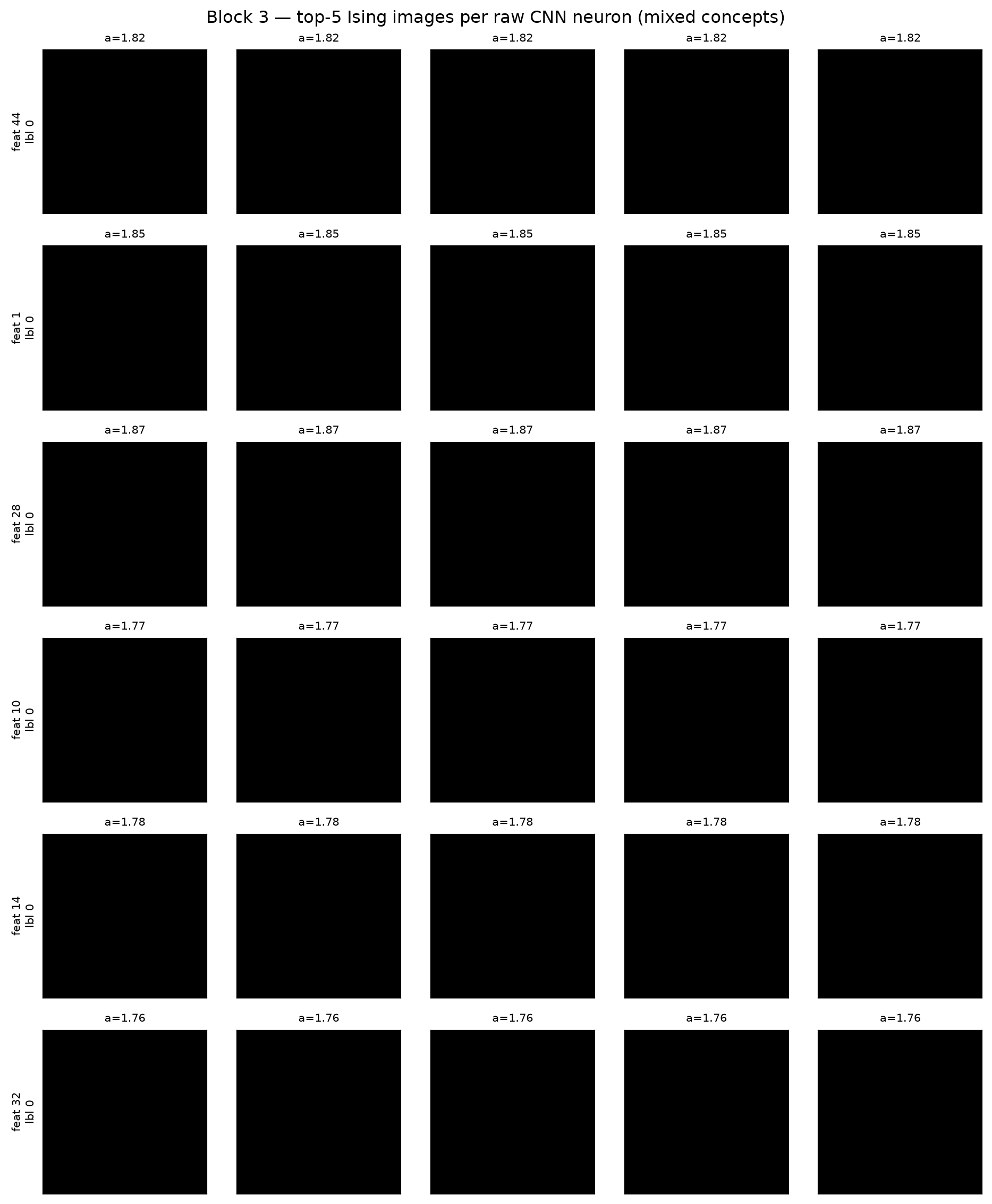
# Top-K activating Ising images per feature, plotted as a grid.# Compare SAE features vs raw neurons of the penultimate layer.TOP_K =5N_FEATS_SHOWN =6# SAE features: pick the most "interesting" — high firing rate but not saturated.with torch.no_grad(): F_vals = sae.encode(H).numpy() # (N, d')sae_score = active.numpy() * (active.numpy() <0.5).astype(float)sae_pick = np.argsort(-sae_score)[:N_FEATS_SHOWN]# Raw neurons: pick by variance (most "informative" axis-aligned units).H_np = H.numpy()raw_pick = np.argsort(-H_np.var(0))[:N_FEATS_SHOWN]def top_k_grid(values: np.ndarray, picks: np.ndarray, title: str):"""values: (N, n_feats). picks: indices into n_feats. Plot rows of TOP_K images.""" fig, axes = plt.subplots(N_FEATS_SHOWN, TOP_K, figsize=(2.0* TOP_K, 2.0* N_FEATS_SHOWN))for row, idx inenumerate(picks): scores = values[:, idx] top = np.argsort(-scores)[:TOP_K]for col, t inenumerate(top): ax = axes[row, col] ax.imshow(X_act[t, 0].numpy(), cmap="gray") ax.set_xticks([]); ax.set_yticks([])if col ==0: ax.set_ylabel(f"feat {idx}\nlbl {int(y_act[t])}", fontsize=8) ax.set_title(f"a={scores[t]:.2f}", fontsize=8) fig.suptitle(title) plt.tight_layout() plt.show()top_k_grid(F_vals, sae_pick, "Block 3 — top-5 Ising images per SAE feature (tend toward one concept)")top_k_grid(H_np, raw_pick, "Block 3 — top-5 Ising images per raw CNN neuron (mixed concepts)")
Read the two grids together. Raw penultimate neurons fire for mixtures of unrelated patterns — high values for both above-Curie and below-Curie images, or for several distinct textures. SAE features, in contrast, tend to concentrate on one concept per feature (e.g. consistently above-Curie, or consistently a particular domain morphology) — the post-ReLU \(\ell_1\) penalty forces the network to spread concepts across many features rather than packing them into shared neurons.
The penalty weight \(\lambda\) tunes the trade-off: too small and features stay polysemantic; too large and many features go dead (never fire). The Anthropic Scaling Monosemanticity report [@templeton_2024_scaling] applied this exact recipe at the scale of a frontier LLM and recovered millions of monosemantic features. This is the Unit-5 autoencoder with \(\ell_1\) on activations, so the connection to the rest of the course is one line of code — every modelling primitive in this lecture is one we have already built.
Block 4 — Counterfactual explanations
Wachter et al. 2017 framed counterfactuals as: given \(x\) with prediction \(f(x) = y\), find the closest\(x'\) such that \(f(x')
\approx y_\text{target}\). Solve by gradient descent on \[
\mathcal{L}_\mathrm{CF}(x') = (f(x') - y_\text{target})^2 + \lambda\, \|x' - x\|_2^2.
\] Pick \(\lambda\) so the data-fit term dominates until the prediction is near target, then the proximity term keeps the perturbation minimal.
We ask: “this 600-°C tensile sample currently predicts 480 MPa. What is the minimum feature change that takes the prediction down to 200 MPa?”
The counterfactual answers a different question than SHAP/IG: not which features mattered, but what would have to be different. It is the natural form of explanation for an engineer looking at a rejected prediction — “if the temperature had been X and the strain Y, the model would have predicted target”. For deployment, this is the most actionable XAI primitive.
Block 5 — Symmetry audit on the Ising classifier
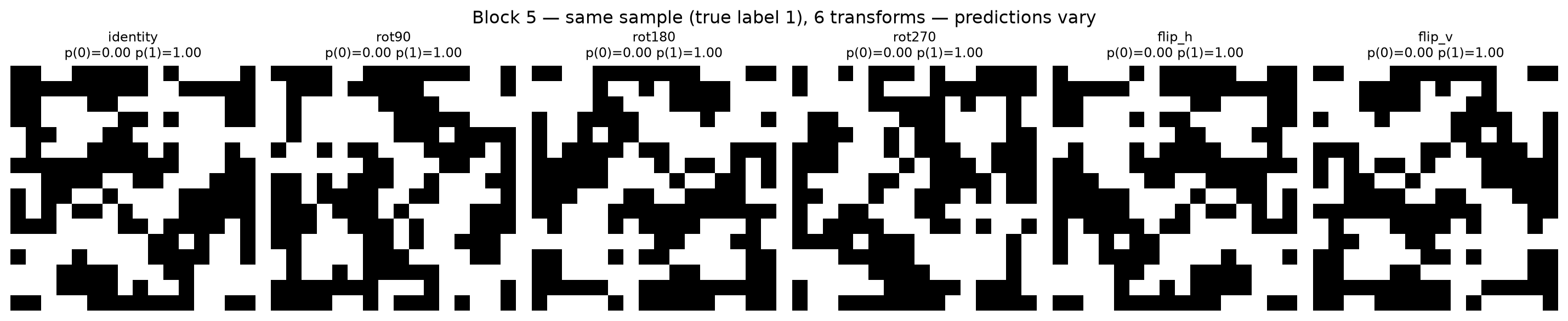
An Ising microstructure is rotation-invariant: the underlying physics (above vs below Curie) does not change if we rotate or flip the image. A classifier should reflect this. CNNs have translation equivariance built in, but not rotation. We measure the gap and repair it with test-time augmentation (TTA): average predictions over the \(\{\)identity, rot90, rot180, rot270, flip-H, flip-V\(\}\) orbit.
# Held-out subset for the audit.torch.manual_seed(0)audit_size =1024audit_idx = torch.randperm(len(ising))[:audit_size]X_aud = ising.X[audit_idx]y_aud = ising.y[audit_idx]ROT_FNS = {"identity": lambda x: x,"rot90": lambda x: torch.rot90(x, k=1, dims=(-2, -1)),"rot180": lambda x: torch.rot90(x, k=2, dims=(-2, -1)),"rot270": lambda x: torch.rot90(x, k=3, dims=(-2, -1)),"flip_h": lambda x: torch.flip(x, dims=(-1,)),"flip_v": lambda x: torch.flip(x, dims=(-2,)),}@torch.no_grad()def acc_under(transform): pred = cnn(transform(X_aud)).argmax(-1)return (pred == y_aud).float().mean().item()print(f"Block 5 — symmetry audit on the Ising CNN ({audit_size} samples):")for name, fn in ROT_FNS.items(): a = acc_under(fn)print(f" {name:<10}: acc = {a:.3f}")# Test-time augmentation: average softmax over the orbit.@torch.no_grad()def tta_predict(x): probs = torch.zeros(len(x), 2)for fn in ROT_FNS.values(): probs += cnn(fn(x)).softmax(-1)return probs /len(ROT_FNS)tta_pred = tta_predict(X_aud).argmax(-1)acc_tta = (tta_pred == y_aud).float().mean().item()print(f" TTA (avg over orbit): acc = {acc_tta:.3f}")
# Visualise predictions under the orbit on one sample.i =0xs = X_aud[i : i +1]fig, axes = plt.subplots(1, 6, figsize=(15, 3.2))for ax, (name, fn) inzip(axes, ROT_FNS.items()): img = fn(xs)[0, 0].numpy()with torch.no_grad(): p = cnn(fn(xs)).softmax(-1)[0] ax.imshow(img, cmap="gray") ax.set_title(f"{name}\np(0)={p[0]:.2f} p(1)={p[1]:.2f}", fontsize=9) ax.axis("off")fig.suptitle(f"Block 5 — same sample (true label {int(y_aud[i])}), 6 transforms — predictions vary")plt.tight_layout()plt.show()
A drop from identity accuracy to rot90 accuracy of even a few percent is not a small bug — it means the model has memorised orientations that the physics says are interchangeable. TTA is a cheap fix at inference time. A more principled fix is to bake the symmetry into the architecture (group-equivariant CNNs, Cohen & Welling 2016) — see week 13’s PIML coverage.
Block 6 — Autoencoder reconstruction error as an OOD detector
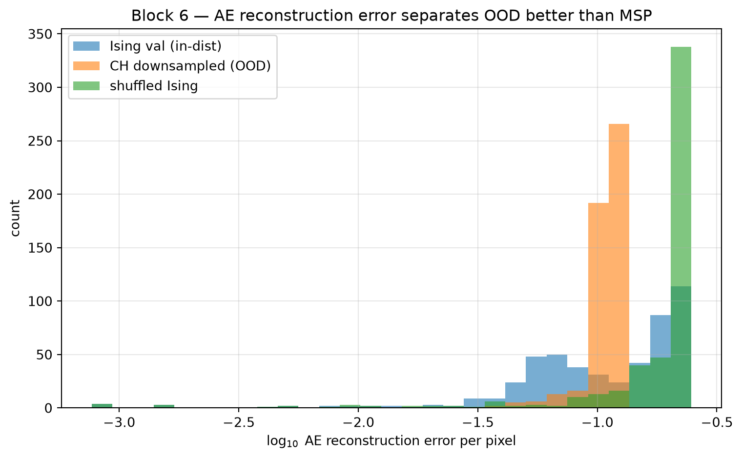
The homework’s max-softmax-probability OOD score is cheap but fragile — it depends on the classifier’s calibration on OOD inputs, which is exactly where calibration is weakest. A more principled detector trains an unsupervised reconstruction model on the in-distribution data; the reconstruction error on OOD inputs is typically much larger because the model has never compressed those patterns.
class TinyAE(nn.Module):def__init__(self, latent: int=16):super().__init__()self.enc = nn.Sequential( nn.Conv2d(1, 16, 3, stride=2, padding=1), nn.GELU(), # 16 -> 8 nn.Conv2d(16, 32, 3, stride=2, padding=1), nn.GELU(), # 8 -> 4 nn.Flatten(), nn.Linear(32*4*4, latent), )self.dec = nn.Sequential( nn.Linear(latent, 32*4*4), nn.GELU(), nn.Unflatten(1, (32, 4, 4)), nn.ConvTranspose2d(32, 16, 4, stride=2, padding=1), nn.GELU(), # 4 -> 8 nn.ConvTranspose2d(16, 1, 4, stride=2, padding=1), # 8 -> 16 )def forward(self, x):returnself.dec(self.enc(x))# Train AE on Ising training split (90% of the dataset).torch.manual_seed(0)n_val_ae =int(0.1*len(ising))n_tr_ae =len(ising) - n_val_aetr_idx, va_idx = torch.utils.data.random_split(range(len(ising)), [n_tr_ae, n_val_ae], generator=torch.Generator().manual_seed(0),)tr_idx =list(tr_idx); va_idx =list(va_idx)ae = TinyAE()opt = torch.optim.AdamW(ae.parameters(), lr=3e-3, weight_decay=1e-4)X_tr_ae = ising.X[tr_idx]print(f"Block 6 — training Ising AE for 5 epochs on {len(X_tr_ae)} samples...")for ep inrange(5): perm = torch.randperm(len(X_tr_ae)) ep_loss =0.0; n =0for i inrange(0, len(perm), 128): b = perm[i : i +128] x = X_tr_ae[b] opt.zero_grad() loss = F.mse_loss(ae(x), x) loss.backward(); opt.step() ep_loss += loss.item() *len(b); n +=len(b)print(f" epoch {ep+1}: train MSE {ep_loss/n:.5f}")@torch.no_grad()def recon_error(x: torch.Tensor, batch: int=256) -> np.ndarray: out = []for i inrange(0, len(x), batch): xb = x[i : i + batch] err = ((ae(xb) - xb) **2).mean(dim=(1, 2, 3)) out.append(err.cpu().numpy())return np.concatenate(out)# Score the three slabs.X_id = ising.X[va_idx] # in-disterr_id = recon_error(X_id)ch = CahnHilliardDataset(simulation_number=0)X_ood_ch = F.avg_pool2d(ch.X, kernel_size=4)[: len(X_id)]err_ch = recon_error(X_ood_ch)X_shuf = X_id.clone()B, C, H, W = X_shuf.shapetorch.manual_seed(0)for i inrange(B): perm = torch.randperm(H * W) flat = X_shuf[i].reshape(C, H * W)[:, perm] X_shuf[i] = flat.reshape(C, H, W)err_shuf = recon_error(X_shuf)print(f"Block 6 — reconstruction error means:")print(f" Ising val: {err_id.mean():.5f}")print(f" CH downsampled: {err_ch.mean():.5f}")print(f" shuffled Ising: {err_shuf.mean():.5f}")# AUROC vs in-dist using reconstruction error as score.y_disc = np.concatenate([np.zeros(len(err_id)), np.ones(len(err_ch))])auc_ch = roc_auc_score(y_disc, np.concatenate([err_id, err_ch]))y_disc = np.concatenate([np.zeros(len(err_id)), np.ones(len(err_shuf))])auc_shuf = roc_auc_score(y_disc, np.concatenate([err_id, err_shuf]))print(f"\nReconstruction-error OOD discrimination AUROC:")print(f" Ising vs CH downsampled: {auc_ch:.3f} (compare to homework MSP)")print(f" Ising vs shuffled Ising: {auc_shuf:.3f}")
Almost always, the AE-reconstruction-error AUROC dominates the homework’s MSP AUROC on the same OOD slabs — the AE was trained to compress in-distribution patterns and refuses to compress OOD ones. The cost is one extra model and a modest amount of training. In a real lab, you would deploy an AE alongside every classifier whose predictions feed an actuator.
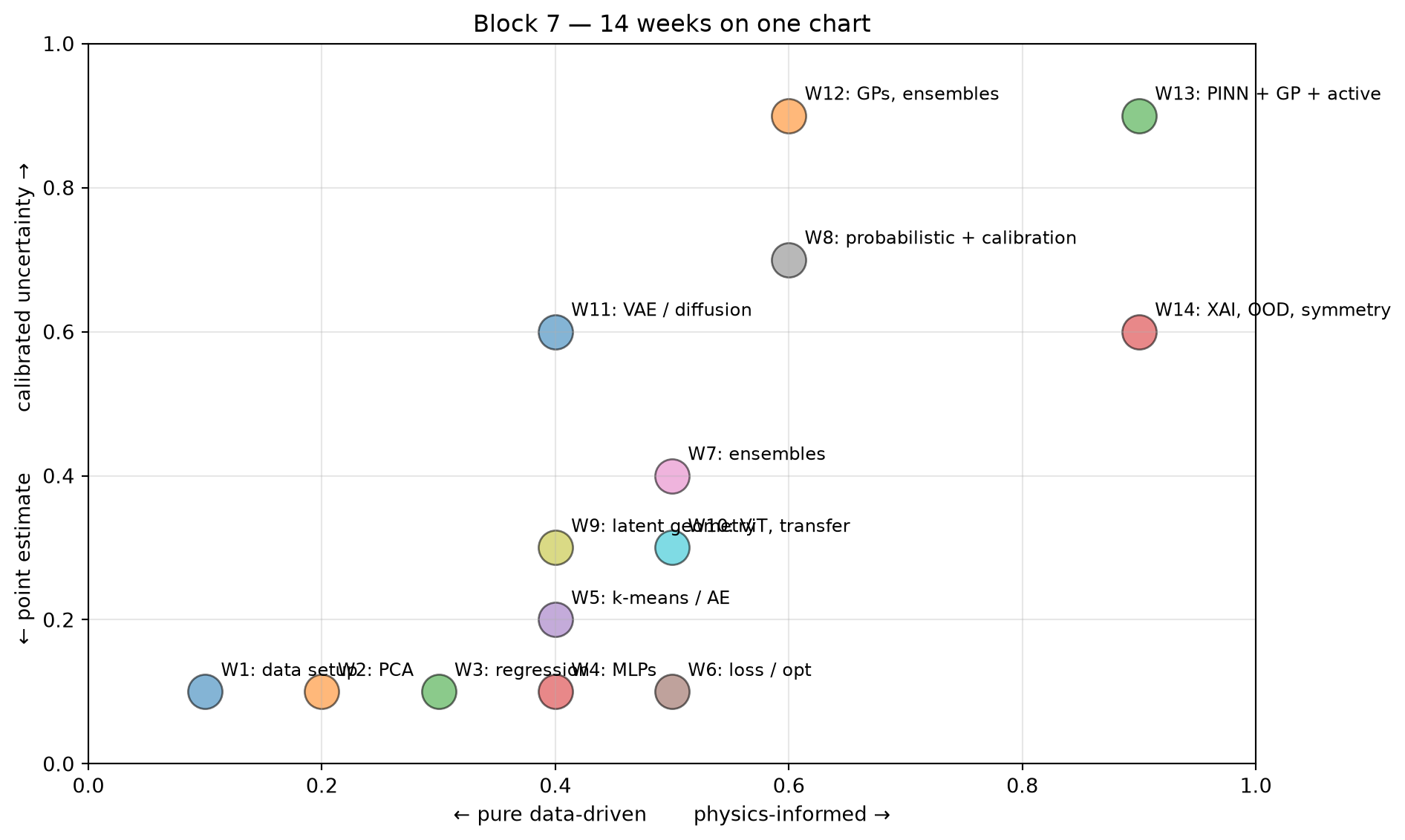
Block 7 — Course retrospective: 14 weeks on one chart
The arc this term: from sparse data to physics-informed uncertainty-aware models.
Course retrospective — methods covered (week → primary method → primary lecture):
  W 1  data + setup                                            [all]
  W 2  linear algebra, PCA                                     [MFML 2 / MG 5]
  W 3  regression as loss min, leakage                         [MFML 3 / ML-PC 3]
  W 4  MLPs, training, baselines (digits, Iris)                [MFML 4 / ML-PC 4-5]
  W 5  k-means + GMM + autoencoders                            [MFML 5 / ML-PC 5]
  W 6  loss landscapes + optimisation + CGNN                   [MFML 6 / MG 6]
  W 7  bias-variance, ensembles, distribution shift            [MFML 7 / ML-PC 8]
  W 8  probabilistic view, MLE/MAP, calibration, robustness    [MFML 8 / MG 8 / ML-PC 8]
  W 9  latent geometry: PCA, t-SNE, contrastive                [MFML 9 / MG 9 / ML-PC 9]
  W10  attention, ViT, cross-system transfer                   [MFML 10 / MG 10 / ML-PC 10]
  W11  VAE / diffusion (generative + inverse design)           [MFML 11 / MG 11 / ML-PC 11]
  W12  uncertainty in predictions, GP, ensembles               [MFML 12 / MG 12 / ML-PC 12]
  W13  PINN + GP + active discovery                            [MFML 13 / MG 13 / ML-PC 13]
  W14  explainability, OOD, symmetry, retrospective            [MFML 14 / MG 14 / ML-PC 14]
# A simple chart: rough conceptual position of each week along two axes.fig, ax = plt.subplots(figsize=(10, 6))data = [# (week, x = data-vs-physics, y = point-vs-uncertainty) (1, 0.1, 0.1, "data setup"), (2, 0.2, 0.1, "PCA"), (3, 0.3, 0.1, "regression"), (4, 0.4, 0.1, "MLPs"), (5, 0.4, 0.2, "k-means / AE"), (6, 0.5, 0.1, "loss / opt"), (7, 0.5, 0.4, "ensembles"), (8, 0.6, 0.7, "probabilistic + calibration"), (9, 0.4, 0.3, "latent geometry"), (10, 0.5, 0.3, "ViT, transfer"), (11, 0.4, 0.6, "VAE / diffusion"), (12, 0.6, 0.9, "GPs, ensembles"), (13, 0.9, 0.9, "PINN + GP + active"), (14, 0.9, 0.6, "XAI, OOD, symmetry"),]for w, x, y, label in data: ax.scatter(x, y, s=300, alpha=0.55, edgecolor="k") ax.annotate(f"W{w}: {label}", (x, y), xytext=(8, 8), textcoords="offset points", fontsize=9)ax.set_xlim(0, 1); ax.set_ylim(0, 1)ax.set_xlabel("← pure data-driven physics-informed →")ax.set_ylabel("← point estimate calibrated uncertainty →")ax.set_title("Block 7 — 14 weeks on one chart")ax.grid(alpha=0.3)plt.tight_layout()plt.show()
Three lessons to walk out the door with:
The right method depends on the data regime. Lots of clean data, no physics → big NN. Sparse data, strong physics → PINN + GP. Distribution shift expected → autoencoder OOD detector deployed alongside.
Uncertainty is not optional in materials work. A point prediction without an uncertainty band is not an answer; it is a promise the model cannot keep. Bayesian regression, deep ensembles, GPs, calibration plots — pick whichever matches the cost-of-a-wrong-answer in your application.
Explainability is a deployment tool, not a research luxury. SHAP / Integrated Gradients / counterfactuals / sparse autoencoders / attention maps each answer a different question. Pick the question first, then pick the method.
Student exercises (Block 8 — ~10 min)
Exercise 1 (core) — SHAP under a different background
Re-run Block 2 with the background set to: (a) all-zeros (the “neutral” baseline), (b) the median tensile sample, and (c) a sample from a different temperature than the query.
How do the SHAP values change? Which background is the right one if the question is “explain this \(T = 600\) prediction relative to what a \(T = 0\) sample would predict”?
The Block 4 counterfactual is the minimum L2 perturbation. Realistic counterfactuals must respect feasibility: \(T\) is one of the three discrete values you can run, strain cannot be negative, etc.
Modify counterfactual so that the strain feature is clipped to its training range and T_norm is projected onto the discrete set \(\{-1, 1/3, 1\}\) corresponding to {0, 400, 600} °C after each gradient step.
Compare to the Block 4 unconstrained CF: how much further does the constrained CF have to travel to achieve the target?
What does a non-feasible counterfactual mean operationally?
# YOUR CODE for Exercise 2 below.
Exercise 3 (core) — Symmetry as a constraint, not a fix
Block 5 used TTA at inference time. A more principled fix is to augment training with rotations and flips. Re-train TinyCNN with on-the-fly random rotations (torch.rot90 with a random k each batch) and random flips. Re-run the symmetry audit. Does the accuracy gap to TTA close?
Bonus: discuss when train-time augmentation is not a good idea (e.g. when the symmetry is approximate, not exact, and breaking it is informative).
# YOUR CODE for Exercise 3 below.
Exercise 4 (stretch) — Calibrated OOD threshold from cost
Block 6 produces a continuous reconstruction-error score. To deploy it, you need a threshold: above this error, refuse to predict.
Pick a cost-of-error model: cost of a false positive (refusing a good prediction) = \(C_\mathrm{FP}\); cost of a false negative (accepting a bad OOD prediction) = \(C_\mathrm{FN}\). Use \(C_\mathrm{FN} = 100 \cdot C_\mathrm{FP}\) as a starting point.
Compute the threshold that minimises expected total cost on the held-out slabs.
Re-run with \(C_\mathrm{FN} / C_\mathrm{FP} = 1, 10, 100, 1000\) and plot threshold vs ratio. Where does the threshold change dramatically — i.e. where does cost asymmetry start to dominate over the score distribution?
# YOUR CODE for Exercise 4 below.
Exam-aligned must-know statements
Re-read these after the exercises; today’s blocks have given you the concrete intuition for every one of them.
Vanilla saliency = \(|x \cdot \partial f_c / \partial x|\). Cheap, biased near saturated activations. (Homework Part A.)
Integrated Gradients = baseline-relative line integral of the gradient. Satisfies completeness and sensitivity. (Homework Part B.)
KernelSHAP = weighted least-squares regression on subsets of “active” vs “background” features, with the Shapley kernel weight. Satisfies efficiency: \(\sum_i \varphi_i = f(x) - f(\text{bg})\). (Block 2.)
Sparse autoencoder (SAE) on a hidden layer = wide encoder + \(\ell_1\) penalty on its post-ReLU code. Lifts polysemantic neurons into monosemantic features. Direct application of superposition[@elhage_2022_superposition] and [@templeton_2024_scaling]. (Block 3.) 4b. Confounder trap. A causally-inert feature correlated with a real driver (campaign/furnace metadata vs \(T\)) gets real SHAP and permutation importance. SHAP is faithful-to-model, not true-of-world. Only an interventiondo(·) (resample the confounder independently of the driver, severing the back-door path) separates prediction from causation. Process chain: composition→processing→microstructure→properties is causal; campaign metadata is merely correlated. (Block 2b.)
Counterfactual = minimum perturbation to flip the prediction; the actionable form of XAI for a deployed model. (Block 4.)
CNNs have translation equivariance built in but not rotation. Test rotation/flip equivariance with an audit and fix with TTA or train-time augmentation. (Block 5.)
Max softmax probability is a cheap OOD detector but fragile, especially against domain-similar OOD. Reconstruction error from an unsupervised AE is a more principled alternative. (Homework Part C, Block 6.)
OOD AUROC of 1.0 means perfect separation, 0.5 means chance. For deployment, pick a threshold by cost-weighted risk, not by AUROC. (Block 6, Exercise 4.)
The right XAI method depends on the question. Why this prediction? → SHAP. Where in the input? → IG/saliency. What would have to change? → counterfactual. What concept does my hidden layer represent? → sparse autoencoder. (All of today.)
The 14-week arc: from data → loss → NN → optimisation → ensembles → probabilistic → representation learning → attention → generative → uncertainty → physics-informed → trust. The destination is deployable, calibrated, explainable models. (Block 7.)