Week 14 — Homework (do BEFORE the Thursday exercise)

This is the final homework of the SS26 sequence. It braids three lectures’ Week 14 content onto a single deployment-audit story.

1. MFML Unit 14 — Explainability, limits, scientific trust. Why XAI; six levels of explainability; sensitivity analysis; SHAP and Integrated Gradients; mechanistic interpretability (sparse autoencoders); OOD detection; counterfactuals.
2. ML-PC Unit 13 — Integration, limits, and reflection. Why ML fails in real labs; explainability for experimental ML (CAMs / SHAP); when ML genuinely changes processing.
3. MG Unit 14 — Physical constraints, limits, and outlook. Stability, charge neutrality, symmetry constraints; what ML can and cannot discover; integration with experimental workflows.

Red thread. A 95%-accurate model has 5% wrong predictions, and the only useful question is which 5%. Today’s homework trains a small Ising classifier, looks under the hood with vanilla input-gradient saliency, fixes the obvious flaw of vanilla saliency with Integrated Gradients, and ends with an out-of-distribution detection check — does the model know when it is being asked to classify something it has never seen? Thursday will then add SHAP, a sparse-autoencoder mechanistic-interpretability audit, counterfactuals, a symmetry audit, an autoencoder OOD detector, and a course retrospective.

Time: ~75 minutes.

What this homework is

Part	Min	Topic	Lecture anchor
A	20	Train a small Ising CNN; vanilla input-gradient saliency on above/below-Curie samples	MFML §“sensitivity analysis”; ML-PC §“CAMs/SHAP for experimental ML”
B	20	Integrated Gradients from scratch; compare to vanilla saliency; why the baseline matters	MFML §“Integrated Gradients”
C	25	OOD detection: max-softmax-probability on Ising (in-dist) vs Cahn-Hilliard (OOD) vs shuffled-pixel (adversarial)	MFML §“limits, OOD detection”; ML-PC §“why ML fails in real labs”
D	10	Reflection: the most expensive failure mode is silent — name one in your area	bridge to Thursday

What you must hand in (or be able to show on Thursday)

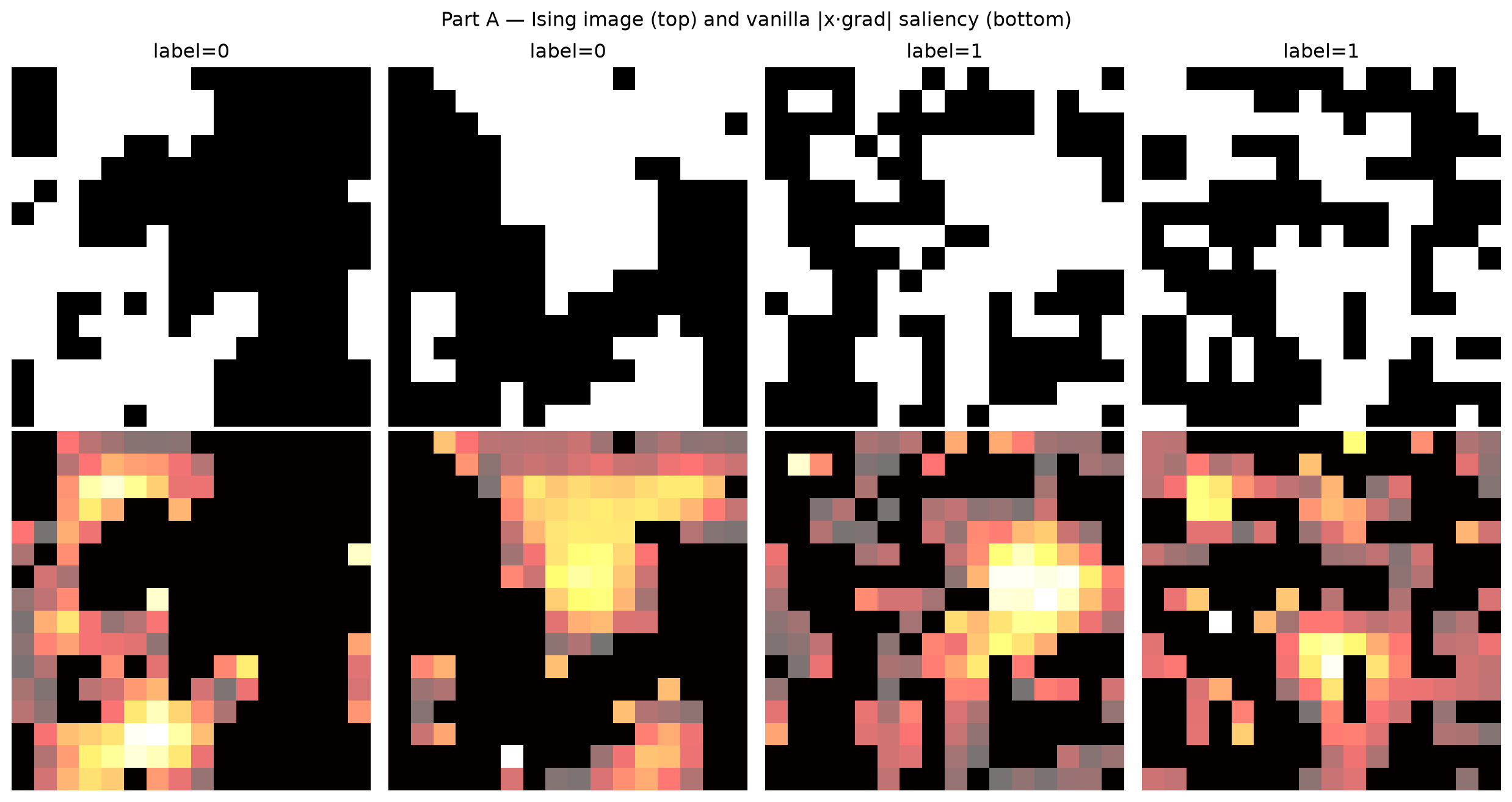
1. Part A: trained CNN val-accuracy + a 4-panel grid showing (image, vanilla saliency) for two above-Curie and two below-Curie samples.
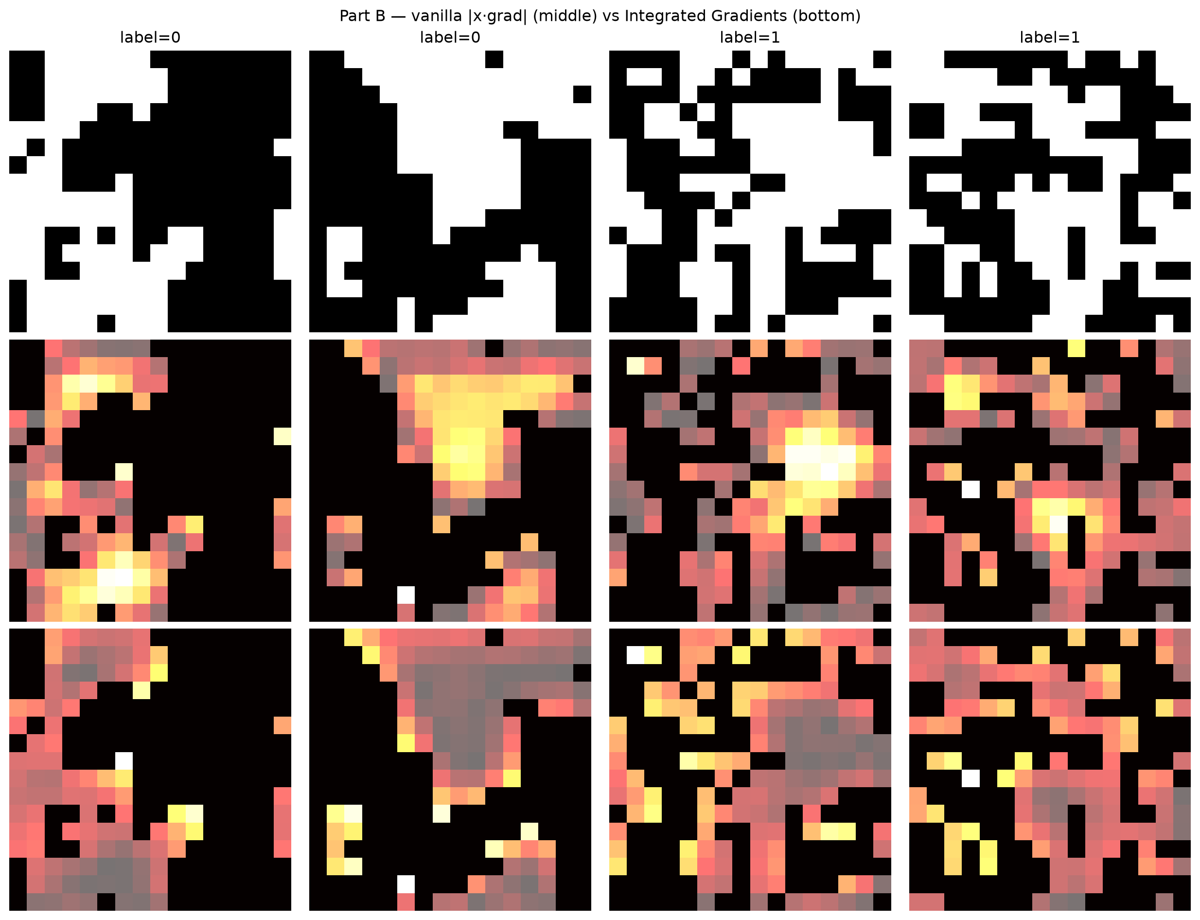
2. Part B: same 4-panel grid but with IG saliency, plus a side- by-side comparison of vanilla vs IG on one sample showing why the baseline matters.
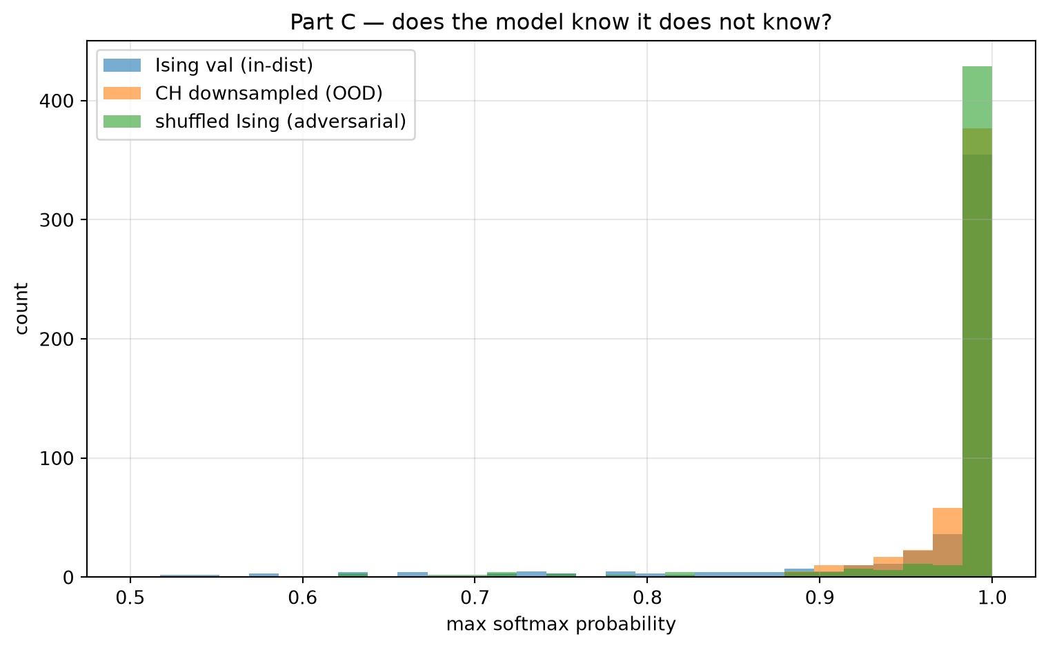
3. Part C: three histograms of max-softmax-probability — Ising test set, Cahn-Hilliard, shuffled-pixel — overlaid; printed AUROC for the (in-dist vs OOD-Cahn-Hilliard) discrimination task.
4. Part D: your reflection paragraph (4-6 sentences).

# Standard imports for the whole homework.
import numpy as np
import torch
import torch.nn as nn
import torch.nn.functional as F
from torch.utils.data import DataLoader, TensorDataset, random_split
import matplotlib.pyplot as plt

from sklearn.metrics import roc_auc_score

from ai4mat.datasets import IsingDataset, CahnHilliardDataset

np.random.seed(0)
torch.manual_seed(0)

<torch._C.Generator at 0x7f0e1c9b6350>

Part A — Train a small Ising CNN, then peek inside with input gradients

Vanilla saliency is the simplest XAI primitive: the absolute value of \(\partial \hat y_c / \partial x\) for the predicted class \(c\) at input \(x\). Big at pixel \(i\) ⇒ infinitesimally moving pixel \(i\) changes the predicted-class logit a lot. It is a one-line torch.autograd.grad call.

We first train a small CNN on Ising-light, then compute vanilla saliency on a few test samples to see what regions of the image the classifier is leaning on.

ising = IsingDataset(size="light")
print(f"Part A — IsingDataset(size='light'): {len(ising)} samples, X {tuple(ising.X.shape)}, y {tuple(ising.y.shape)}")
print(f"  class balance: {torch.bincount(ising.y).tolist()}")


class TinyCNN(nn.Module):
    def __init__(self, n_classes: int = 2):
        super().__init__()
        self.net = nn.Sequential(
            nn.Conv2d(1, 16, 3, padding=1), nn.GELU(),
            nn.Conv2d(16, 32, 3, padding=1), nn.GELU(),
            nn.Conv2d(32, 64, 3, padding=1), nn.GELU(),
            nn.AdaptiveAvgPool2d(1), nn.Flatten(),
            nn.Linear(64, n_classes),
        )

    def forward(self, x):
        return self.net(x)


# Train/val split.
torch.manual_seed(0)
n_val = int(0.1 * len(ising))
n_tr = len(ising) - n_val
tr, va = random_split(ising, [n_tr, n_val],
                     generator=torch.Generator().manual_seed(0))
tr_dl = DataLoader(tr, batch_size=128, shuffle=True)
va_dl = DataLoader(va, batch_size=128, shuffle=False)

cnn = TinyCNN()
opt = torch.optim.AdamW(cnn.parameters(), lr=3e-3, weight_decay=1e-4)
N_EPOCHS = 5
print(f"Training TinyCNN for {N_EPOCHS} epochs...")
for ep in range(N_EPOCHS):
    cnn.train()
    ep_loss = ep_n = 0
    for xb, yb in tr_dl:
        opt.zero_grad()
        loss = F.cross_entropy(cnn(xb), yb)
        loss.backward(); opt.step()
        ep_loss += loss.item() * len(yb); ep_n += len(yb)
    cnn.eval()
    correct = total = 0
    with torch.no_grad():
        for xb, yb in va_dl:
            correct += (cnn(xb).argmax(-1) == yb).sum().item()
            total += len(yb)
    print(f"  epoch {ep+1}: train loss {ep_loss/ep_n:.4f} | val acc {correct/total:.3f}")

Part A — IsingDataset(size='light'): 5000 samples, X (5000, 1, 16, 16), y (5000,)
  class balance: [2507, 2493]
Training TinyCNN for 5 epochs...
  epoch 1: train loss 0.4582 | val acc 0.956
  epoch 2: train loss 0.1311 | val acc 0.942
  epoch 3: train loss 0.1784 | val acc 0.948
  epoch 4: train loss 0.1218 | val acc 0.956
  epoch 5: train loss 0.1166 | val acc 0.962

def vanilla_saliency(model, x: torch.Tensor) -> np.ndarray:
    """|x . d logit_class / dx|, where class is the model's prediction.

    Returns saliency per pixel, normalised to [0, 1] per sample.
    """
    model.eval()
    x = x.clone().requires_grad_(True)
    logits = model(x)
    pred = logits.argmax(-1)
    sel = logits.gather(1, pred.unsqueeze(1)).sum()
    sel.backward()
    sal = (x.grad * x.detach()).abs().squeeze(1).numpy()
    sal = sal / (sal.max(axis=(1, 2), keepdims=True) + 1e-12)
    return sal


# Pick 2 above-Curie and 2 below-Curie samples.
labels_np = ising.y.numpy()
i_below = np.where(labels_np == 0)[0][:2]
i_above = np.where(labels_np == 1)[0][:2]
idx = np.concatenate([i_below, i_above])
imgs = ising.X[idx]
labels = ising.y[idx]
sal_van = vanilla_saliency(cnn, imgs)
print(f"Part A — vanilla saliency shape: {sal_van.shape}")

Part A — vanilla saliency shape: (4, 16, 16)

fig, axes = plt.subplots(2, 4, figsize=(13, 7))
for i in range(4):
    axes[0, i].imshow(imgs[i, 0].numpy(), cmap="gray")
    axes[0, i].set_title(f"label={labels[i].item()}")
    axes[0, i].axis("off")
    axes[1, i].imshow(imgs[i, 0].numpy(), cmap="gray")
    axes[1, i].imshow(sal_van[i], cmap="hot", alpha=0.55)
    axes[1, i].axis("off")
fig.suptitle("Part A — Ising image (top) and vanilla |x·grad| saliency (bottom)")
plt.tight_layout()
plt.show()

Part A deliverable: the 8-panel figure above.

Vanilla saliency tells you where the prediction is locally sensitive — but it has a known weakness: at any saturated activation (ReLU, GELU, sigmoid in the middle) the gradient is small even when that pixel was causally important for crossing the threshold. Part B fixes this with Integrated Gradients.

Part B — Integrated Gradients

Integrated Gradients (Sundararajan et al. 2017) uses the gradient along a path from a reference baseline \(x'\) to the input \(x\): \[ \mathrm{IG}_i(x) = (x_i - x'_i) \cdot \int_0^1 \frac{\partial f_c(x' + \alpha (x - x'))}{\partial x_i}\, d\alpha, \] discretised to a Riemann sum over \(K\) steps. The baseline is the question “relative to what is this pixel important?”: for grayscale microstructures a black image \(x' = 0\) or the dataset mean image both make sense.

IG satisfies two properties vanilla saliency does not:

1. Completeness: \(\sum_i \mathrm{IG}_i(x) = f_c(x) - f_c(x')\).
2. Sensitivity: if input and baseline differ in one feature and that feature changes the output, IG attributes a non-zero score.

def integrated_gradients(model, x: torch.Tensor, baseline: torch.Tensor,
                         n_steps: int = 32) -> np.ndarray:
    """IG attribution per pixel for the predicted class.

    Returns saliency normalised to [0, 1] per sample.
    """
    model.eval()
    with torch.no_grad():
        pred = model(x).argmax(-1)
    grads = torch.zeros_like(x)
    for k in range(1, n_steps + 1):
        alpha = k / n_steps
        x_alpha = (baseline + alpha * (x - baseline)).clone().requires_grad_(True)
        logits = model(x_alpha)
        sel = logits.gather(1, pred.unsqueeze(1)).sum()
        sel.backward()
        grads = grads + x_alpha.grad
    avg_grad = grads / n_steps
    ig = (x - baseline) * avg_grad
    sal = ig.abs().squeeze(1).numpy()
    sal = sal / (sal.max(axis=(1, 2), keepdims=True) + 1e-12)
    return sal


baseline = torch.zeros_like(imgs)
sal_ig = integrated_gradients(cnn, imgs, baseline)

fig, axes = plt.subplots(3, 4, figsize=(13, 10))
for i in range(4):
    axes[0, i].imshow(imgs[i, 0].numpy(), cmap="gray")
    axes[0, i].set_title(f"label={labels[i].item()}")
    axes[0, i].axis("off")
    axes[1, i].imshow(imgs[i, 0].numpy(), cmap="gray")
    axes[1, i].imshow(sal_van[i], cmap="hot", alpha=0.55)
    axes[1, i].axis("off")
    axes[2, i].imshow(imgs[i, 0].numpy(), cmap="gray")
    axes[2, i].imshow(sal_ig[i], cmap="hot", alpha=0.55)
    axes[2, i].axis("off")
axes[1, 0].set_ylabel("vanilla")
axes[2, 0].set_ylabel("IG")
fig.suptitle("Part B — vanilla |x·grad| (middle) vs Integrated Gradients (bottom)")
plt.tight_layout()
plt.show()

# Verify the completeness axiom on one sample: sum of IG ≈ f_c(x) - f_c(x').
i_test = 0
x_one = imgs[i_test : i_test + 1]
b_one = baseline[i_test : i_test + 1]
with torch.no_grad():
    fx = cnn(x_one).softmax(-1)[0]
    fb = cnn(b_one).softmax(-1)[0]
    pred_class = int(cnn(x_one).argmax(-1))

ig_one = integrated_gradients(cnn, x_one, b_one)
# Re-do without normalisation to check completeness in raw units.
n_steps = 64
grads = torch.zeros_like(x_one)
for k in range(1, n_steps + 1):
    alpha = k / n_steps
    x_alpha = (b_one + alpha * (x_one - b_one)).clone().requires_grad_(True)
    logits = cnn(x_alpha)
    sel = logits.gather(1, torch.tensor([[pred_class]])).sum()
    sel.backward()
    grads = grads + x_alpha.grad
avg_grad = grads / n_steps
ig_raw = ((x_one - b_one) * avg_grad).sum().item()
delta_logit = (cnn(x_one)[0, pred_class] - cnn(b_one)[0, pred_class]).item()
print(f"\nPart B — completeness check on sample 0 (predicted class {pred_class}):")
print(f"  sum of IG_i (logit space)         = {ig_raw:>10.4f}")
print(f"  f_c(x) - f_c(baseline)            = {delta_logit:>10.4f}")
print(f"  difference (Riemann discretisation): {abs(ig_raw - delta_logit):.4f}")

Part B — completeness check on sample 0 (predicted class 0):
  sum of IG_i (logit space)         =    -5.7169
  f_c(x) - f_c(baseline)            =    -5.9254
  difference (Riemann discretisation): 0.2085

Part B deliverable: the three-row comparison figure and the completeness-check printout.

IG often produces a less peaky attribution than vanilla — the integration smooths over saturated activations and gives credit to every pixel along the path. The completeness sanity check should match to within Riemann discretisation error (a few percent at n_steps=64).

Part C — Out-of-distribution detection: does the model know it

does not know?

A model trained only on Ising will still output a confident prediction when handed a Cahn-Hilliard image or a shuffled-pixel noise pattern. The maximum softmax probability (MSP) is a cheap baseline for “how confident is the model?” — we compute it on three slabs and compare:

• Ising test set (in-distribution).
• Cahn-Hilliard images, downsampled to 16×16 (OOD-similar).
• Shuffled Ising (every pixel of an Ising image scrambled into a random order — same marginal pixel distribution as Ising, but the spatial structure is destroyed).

A trustworthy model should be less confident on OOD slabs than on the in-distribution slab.

@torch.no_grad()
def msp(model, x: torch.Tensor, batch: int = 256) -> np.ndarray:
    """Maximum softmax probability per sample."""
    model.eval()
    out = []
    for i in range(0, len(x), batch):
        out.append(model(x[i : i + batch]).softmax(-1).max(-1).values.cpu().numpy())
    return np.concatenate(out)


# (a) in-distribution: Ising val split.
X_id = torch.stack([va[i][0] for i in range(len(va))])
msp_id = msp(cnn, X_id)
print(f"Part C — MSP on:")
print(f"  Ising val ({len(X_id)} samples):        mean = {msp_id.mean():.3f}")

# (b) OOD same-domain: Cahn-Hilliard, single simulation, downsampled to 16×16.
ch = CahnHilliardDataset(simulation_number=0)
X_ood_ch = F.avg_pool2d(ch.X, kernel_size=4)[: len(X_id)]
msp_ch = msp(cnn, X_ood_ch)
print(f"  CH downsampled ({len(X_ood_ch)}):      mean = {msp_ch.mean():.3f}")

# (c) OOD adversarial: shuffle Ising pixels.
torch.manual_seed(0)
X_shuf = X_id.clone()
B, C, H, W = X_shuf.shape
for i in range(B):
    perm = torch.randperm(H * W)
    flat = X_shuf[i].reshape(C, H * W)[:, perm]
    X_shuf[i] = flat.reshape(C, H, W)
msp_shuf = msp(cnn, X_shuf)
print(f"  shuffled Ising ({len(X_shuf)}):       mean = {msp_shuf.mean():.3f}")

Part C — MSP on:
  Ising val (500 samples):        mean = 0.959
  CH downsampled (500):      mean = 0.985
  shuffled Ising (500):       mean = 0.978

# Histograms.
fig, ax = plt.subplots(figsize=(8, 5))
bins = np.linspace(0.5, 1.0, 30)
ax.hist(msp_id, bins=bins, alpha=0.6, label="Ising val (in-dist)")
ax.hist(msp_ch, bins=bins, alpha=0.6, label="CH downsampled (OOD)")
ax.hist(msp_shuf, bins=bins, alpha=0.6, label="shuffled Ising (adversarial)")
ax.set_xlabel("max softmax probability")
ax.set_ylabel("count")
ax.set_title("Part C — does the model know it does not know?")
ax.grid(alpha=0.3); ax.legend()
plt.tight_layout()
plt.show()

# AUROC for distinguishing in-dist from CH OOD using -MSP as score.
y_disc = np.concatenate([np.zeros(len(msp_id)), np.ones(len(msp_ch))])
score_disc = np.concatenate([-msp_id, -msp_ch])
auc_ch = roc_auc_score(y_disc, score_disc)
y_disc2 = np.concatenate([np.zeros(len(msp_id)), np.ones(len(msp_shuf))])
score_disc2 = np.concatenate([-msp_id, -msp_shuf])
auc_shuf = roc_auc_score(y_disc2, score_disc2)
print(f"\nMSP-based OOD discrimination AUROC:")
print(f"  Ising vs Cahn-Hilliard:    {auc_ch:.3f}    (1.0 = perfect, 0.5 = chance)")
print(f"  Ising vs shuffled Ising:   {auc_shuf:.3f}")

MSP-based OOD discrimination AUROC:
  Ising vs Cahn-Hilliard:    0.505    (1.0 = perfect, 0.5 = chance)
  Ising vs shuffled Ising:   0.246

Part C deliverable: the histogram figure and the two AUROC numbers.

Two failure modes you can read off the figure:

• If the Cahn-Hilliard MSP histogram overlaps the in-dist histogram heavily (AUROC near 0.5), MSP is not a usable OOD detector for that domain shift — the classifier is confidently wrong.
• If the shuffled MSP is high (model still confident on nonsense), the model has not learned anything that depends on spatial structure — it is just exploiting pixel marginals.
• Thursday Block 6 builds an autoencoder-reconstruction OOD detector that fixes both of these failure modes.

Part D — Reflection: the most expensive failure mode is silent

A model that flags its own uncertainty is recoverable; a model that is confidently wrong on out-of-distribution inputs costs experiments, wafers, beam time, or — in deployment — public trust.

Your task (~10 min, write 4-6 sentences):

Pick one materials scenario in your area (microscopy, processing, a property predictor) and answer two questions:

1. Which “OOD” matters most? Be specific: what kind of input does the model occasionally see in production that it never saw in training? Examples: a different sample preparation, an instrument that drifted, a new alloy family, a different vendor’s feedstock, a chemical contaminant.
2. What is the cost of one silent wrong prediction? Quantify if you can: hours of beam time, kilograms of feedstock, a wrong process recommendation that proliferates, a paper retraction, a contractual obligation. The number does not have to be exact — the order of magnitude is what matters when you are choosing a threshold for “the model should refuse to answer”.

Bring the paragraph to Thursday; we will pick two volunteers to read theirs aloud at the start of Block 1.

Hand in: your written paragraph (Markdown cell below).

(your reflection paragraph here)