Week 3 — Homework (do BEFORE the Thursday exercise)
This notebook is the mandatory warm-up for the Week 3 in-class exercise. Working through it gets the ai4mat install pain out of the way, gives everyone the same PyTorch baseline to talk about, and primes you for the basis-functions story we unfold in class.
Time: ~75 minutes.
What this homework is
Three short workouts, all anchored on the same idea:
A “linear” model is linear in its parameters, not in its features. Polynomial, spline, Fourier, and wavelet models all live inside the same loss-minimisation framework — they only differ in which basis functions you choose.
Part
Min
Topic
Lecture anchor
A
30
PyTorch baseline on a real materials dataset
MFML §“supervised learning framework”
B
25
FFT — frequency content as a basis
ML-PC §18
C
15
Wavelets — when the basis must be local
ML-PC §19
D
5
Reflection paragraph linking A→B→C
bridge to Thursday’s class
What you must hand in (or be able to show on Thursday)
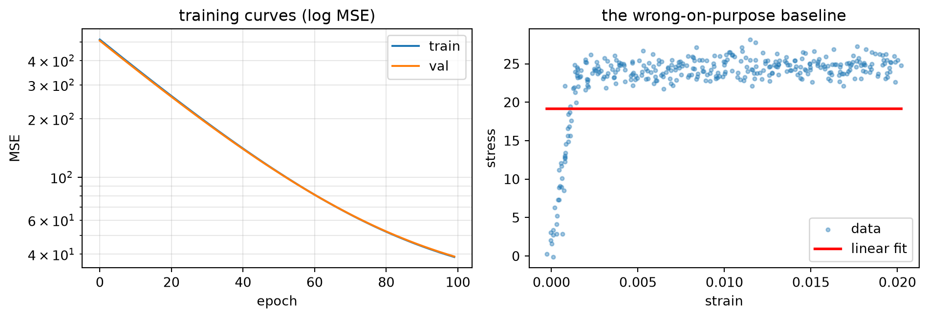
Train/val MSE curves from Part A.
Spectrum + reconstruction figure from Part B.
Scalogram + FFT comparison figure from Part C.
Your written answer to the reflection question (Part D).
# Standard imports for the whole homework. Same seeds idiom as week 2.import numpy as npimport torchimport torch.nn as nnfrom torch.utils.data import DataLoader, random_splitimport matplotlib.pyplot as pltfrom ai4mat.datasets import TensileTestDatasetnp.random.seed(0)torch.manual_seed(0)
<torch._C.Generator at 0x7fcd317b98d0>
Part A — PyTorch baseline on TensileTestDataset
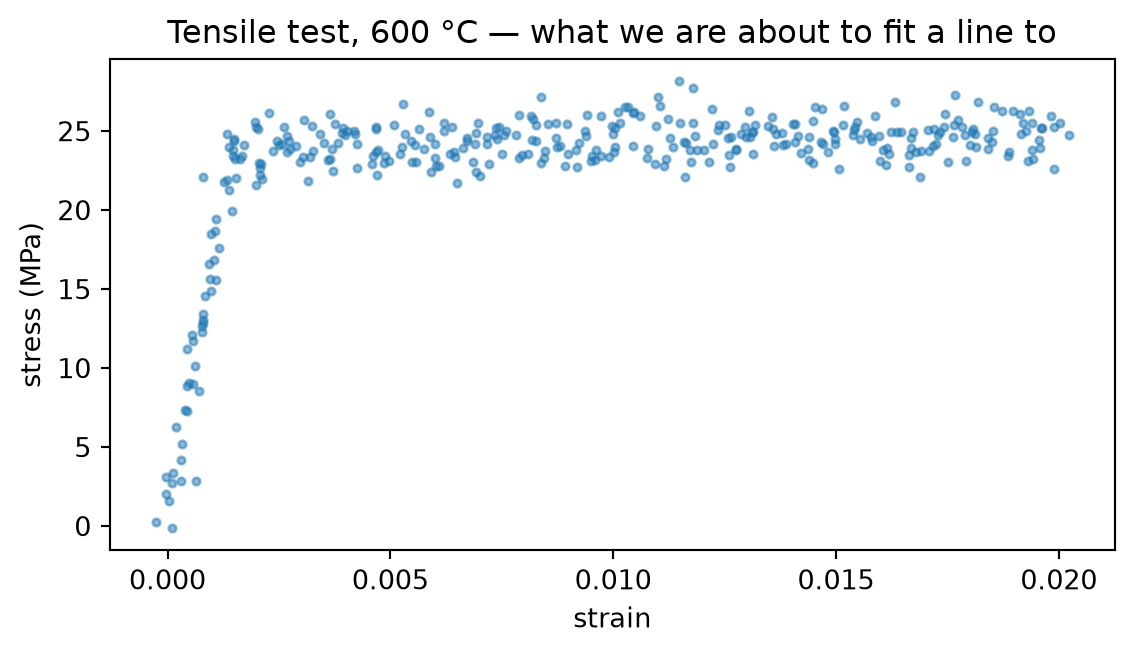
We fit a 1-feature linear model stress = w * strain + b to a tensile-test stress–strain curve at 600 °C. The dataset is small (350 samples), the model has 2 parameters, and the loss is MSE. Everything is intentionally minimal — this is the strawman that the in-class notebook will then break apart and improve.
# Load the data and look at it.dataset = TensileTestDataset(temperature=600)print(f"Dataset size: {len(dataset)}")x0, y0 = dataset[0]print(f"Sample 0: strain={float(x0):.4f} stress={float(y0):.2f} MPa")X_all = torch.stack([dataset[i][0] for i inrange(len(dataset))]).squeeze(1) # (N,)y_all = torch.stack([dataset[i][1] for i inrange(len(dataset))]) # (N,)plt.figure(figsize=(6, 3.5))plt.scatter(X_all.numpy(), y_all.numpy(), s=8, alpha=0.5)plt.xlabel("strain"); plt.ylabel("stress (MPa)")plt.title("Tensile test, 600 °C — what we are about to fit a line to")plt.tight_layout(); plt.show()
Notice the curve is not a line — it has an elastic regime, a yield knee, and a work-hardening tail. A linear model is wrong for this data, on purpose. Part A establishes the wrong baseline; the in-class notebook will fix it with bases that can express curvature.
# Train/val split with a fixed generator so the split is reproducible.gen = torch.Generator().manual_seed(0)n_train =int(0.8*len(dataset))n_val =len(dataset) - n_traintrain_ds, val_ds = random_split(dataset, [n_train, n_val], generator=gen)train_loader = DataLoader(train_ds, batch_size=32, shuffle=True, generator=torch.Generator().manual_seed(0))val_loader = DataLoader(val_ds, batch_size=32, shuffle=False)print(f"train={n_train} val={n_val}")
train=280 val=70
class LinearModel(nn.Module):def__init__(self):super().__init__()self.linear = nn.Linear(1, 1)def forward(self, x):returnself.linear(x).squeeze(-1)model = LinearModel()print(model)print("params:", sum(p.numel() for p in model.parameters()))
Hold on to the train/val MSE numbers above — Block 1 of the in-class notebook will check that closed-form OLS lands on the same answer to within numerical precision.
Part B — FFT as a basis-function expansion
Question: if a “linear” model is allowed any basis we like, what does it look like to choose the Fourier basis?
Answer: for a periodic signal sampled at \(N\) points, the discrete Fourier transform is exactly the least-squares projection onto the basis \(\{\sin(2\pi k t / T),\ \cos(2\pi k t / T)\}_{k=0}^{N/2}\).
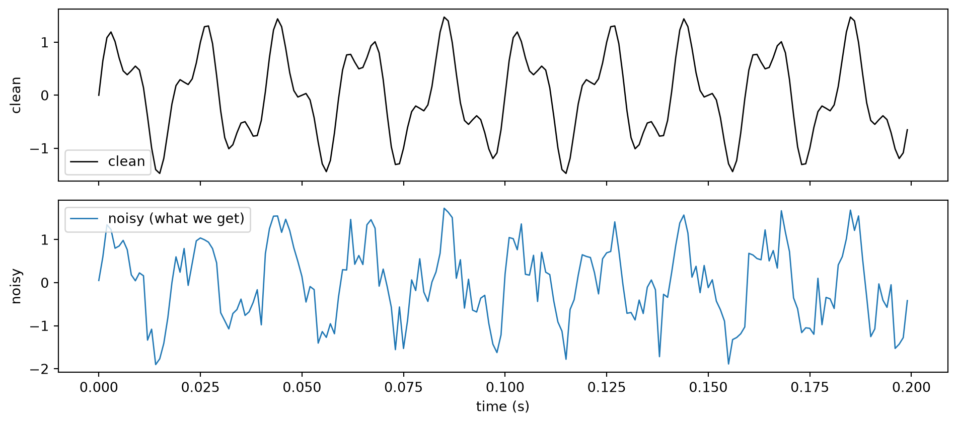
The FFT is therefore “linear regression on the Fourier basis”, computed in \(\mathcal{O}(N \log N)\) instead of \(\mathcal{O}(N^3)\). Below we make this concrete on a noisy two-tone signal.
# Synthetic signal: two pure tones plus white noise.fs =1000.0# sampling rate, HzT =1.0# 1 second of datat = np.arange(0, T, 1/fs) # (N,)N = t.sizef1, f2 =50.0, 120.0# the two true frequenciesclean =1.0*np.sin(2*np.pi*f1*t) +0.5*np.sin(2*np.pi*f2*t)noise = np.random.default_rng(0).normal(0.0, 0.4, size=N)signal = clean + noisefig, ax = plt.subplots(2, 1, figsize=(10, 4.5), sharex=True)ax[0].plot(t[:200], clean[:200], 'k', lw=1, label="clean")ax[0].set_ylabel("clean"); ax[0].legend()ax[1].plot(t[:200], signal[:200], 'tab:blue', lw=1, label="noisy (what we get)")ax[1].set_xlabel("time (s)"); ax[1].set_ylabel("noisy"); ax[1].legend()plt.tight_layout(); plt.show()
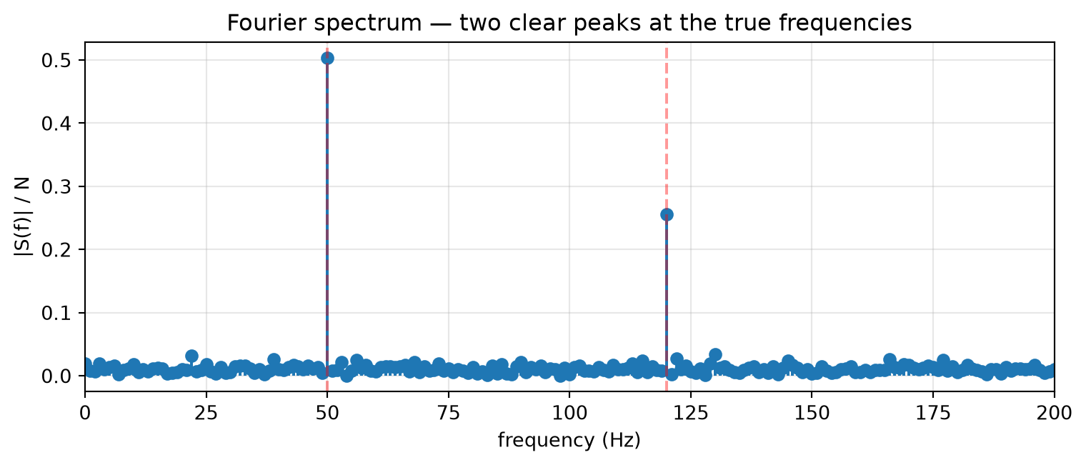
# FFT magnitude spectrum.S = np.fft.rfft(signal)freqs = np.fft.rfftfreq(N, 1/fs)mag = np.abs(S) / Nplt.figure(figsize=(8, 3.5))plt.stem(freqs, mag, basefmt=" ")plt.xlim(0, 200); plt.xlabel("frequency (Hz)"); plt.ylabel("|S(f)| / N")plt.title("Fourier spectrum — two clear peaks at the true frequencies")plt.axvline(f1, color='r', linestyle='--', alpha=0.4)plt.axvline(f2, color='r', linestyle='--', alpha=0.4)plt.grid(alpha=0.3); plt.tight_layout(); plt.show()
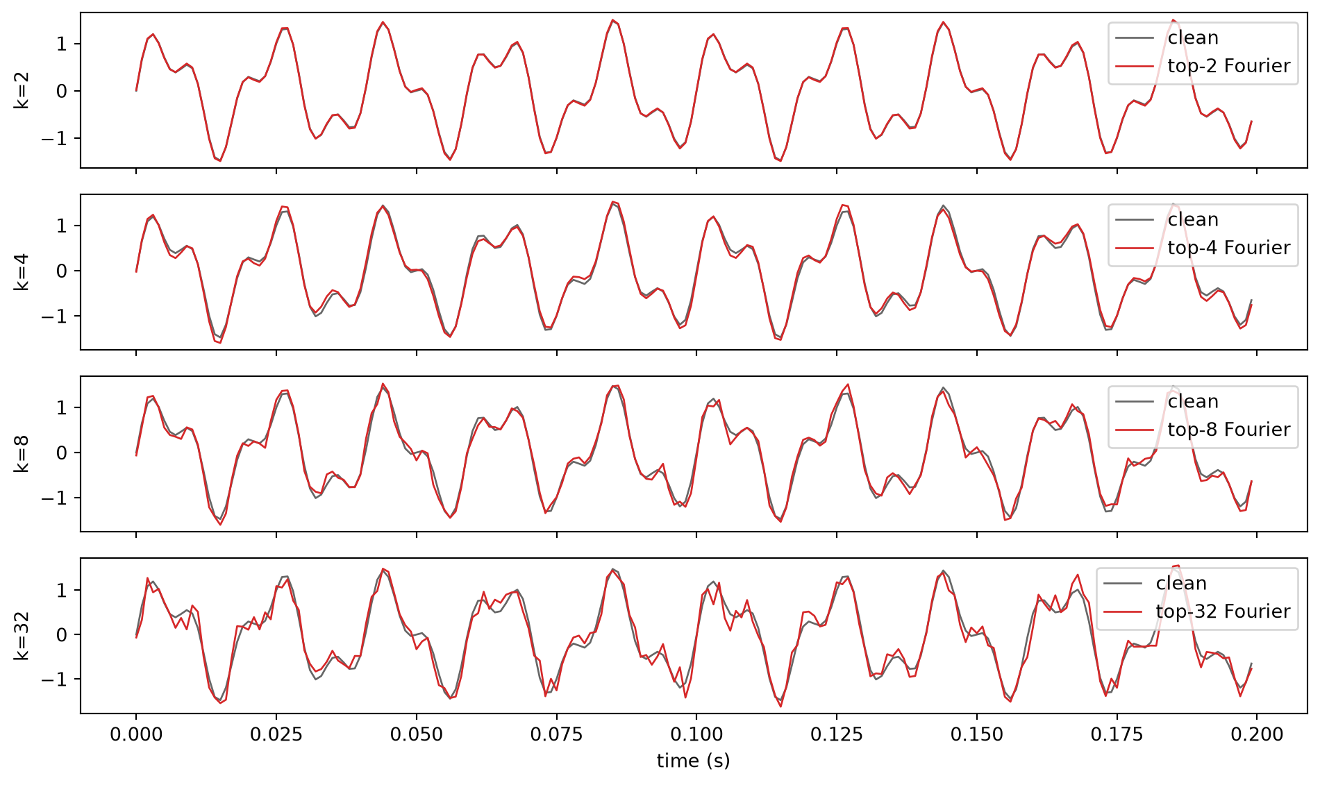
# Reconstruct from the top-k Fourier coefficients (a.k.a. low-rank denoising in# the Fourier basis -- exactly the SVD truncation idea from week 2, with the# basis fixed in advance).def topk_reconstruct(signal, k): S = np.fft.rfft(signal) keep = np.argsort(np.abs(S))[-k:] # indices of the k largest coefficients S_trunc = np.zeros_like(S) S_trunc[keep] = S[keep]return np.fft.irfft(S_trunc, n=signal.size)ks = [2, 4, 8, 32]fig, ax = plt.subplots(len(ks), 1, figsize=(10, 6), sharex=True)for a, k inzip(ax, ks): rec = topk_reconstruct(signal, k) a.plot(t[:200], clean[:200], 'k', lw=1, alpha=0.6, label="clean") a.plot(t[:200], rec[:200], 'tab:red', lw=1, label=f"top-{k} Fourier") a.legend(loc='upper right'); a.set_ylabel(f"k={k}")ax[-1].set_xlabel("time (s)")plt.tight_layout(); plt.show()
Reading the picture: keep the top 2 Fourier coefficients and you already recover the two-tone signal almost perfectly — because the true signal is rank-2 in the Fourier basis. A polynomial fit would need many more parameters to do this, because polynomials are a bad basis for periodic data.
Take-away:which basis you pick is itself a modelling choice. Pick the one whose coefficients are sparse for your signal class.
Part C — Wavelets: when the basis must be local
The FFT reads a signal as an infinite stack of pure sines. That works perfectly when the signal is genuinely periodic. But what if the interesting event is a transient burst at one moment in time — a defect avalanche, a phase pop, a delamination click? Sines are infinite in time; they cannot localise a burst.
Wavelets are a localised basis: each wavelet has both a frequency and a location. The continuous wavelet transform (CWT) gives you a 2-D scalogram of “how much of frequency \(f\) is present at time \(t\)”.
# Install the wavelet library (uncomment if running in a fresh env or Colab).# !pip install pywaveletsimport pywt # noqa: E402
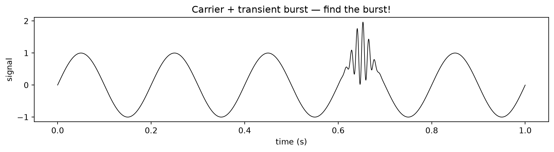
# Synthetic signal: low-frequency carrier + a Gaussian-windowed high-frequency burst.# Variables here are namespaced with `_c` so they don't shadow Part B's `t`, `fs`, `signal`, `S`.t_c = np.linspace(0, 1.0, 2000)fs_c =1.0/ (t_c[1] - t_c[0])carrier = np.sin(2*np.pi*5*t_c) # 5 Hz backgroundburst = np.exp(-((t_c -0.65)/0.02)**2) * np.sin(2*np.pi*80*t_c) # 80 Hz pulse @ t=0.65ssignal_c = carrier + burstplt.figure(figsize=(10, 2.8))plt.plot(t_c, signal_c, 'k', lw=0.8); plt.xlabel("time (s)"); plt.ylabel("signal")plt.title("Carrier + transient burst — find the burst!"); plt.tight_layout(); plt.show()
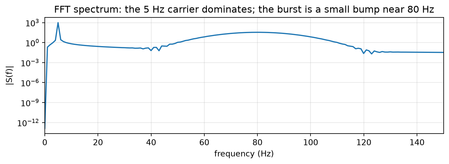
# FFT view: the burst smears across the spectrum.S_c = np.fft.rfft(signal_c)freqs_c = np.fft.rfftfreq(t_c.size, 1/fs_c)plt.figure(figsize=(8, 3))plt.semilogy(freqs_c, np.abs(S_c))plt.xlim(0, 150); plt.xlabel("frequency (Hz)"); plt.ylabel("|S(f)|")plt.title("FFT spectrum: the 5 Hz carrier dominates; the burst is a small bump near 80 Hz")plt.grid(alpha=0.3); plt.tight_layout(); plt.show()
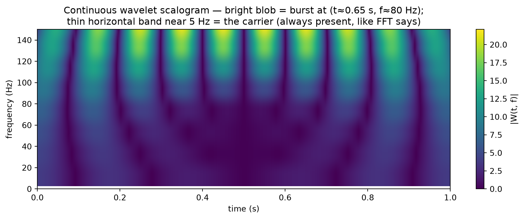
# CWT view: the burst pops out at exactly the right (time, frequency).# Scale range is chosen so freqs_cwt covers ~3 Hz (below the 5 Hz carrier) up to# ~150 Hz (above the 80 Hz burst). For the Morlet wavelet, scale s maps to# frequency f ≈ 0.8125 / (s * dt), so larger s = lower f.scales = np.geomspace(1, 600, 80)coeffs, freqs_cwt = pywt.cwt(signal_c, scales=scales, wavelet="morl", sampling_period=1/fs_c)# `coeffs` is ordered (smallest scale = highest freq) at row 0. Use origin='upper'# so row 0 lands at the TOP of the image, matching the extent's high-freq-on-top.plt.figure(figsize=(10, 4))plt.imshow(np.abs(coeffs), aspect="auto", origin="upper", extent=[t_c[0], t_c[-1], freqs_cwt[-1], freqs_cwt[0]], cmap="viridis")plt.ylim(0, 150) # crop the empty high-freq band so the burst dominates the figureplt.xlabel("time (s)"); plt.ylabel("frequency (Hz)")plt.title("Continuous wavelet scalogram — bright blob = burst at (t≈0.65 s, f≈80 Hz);\n""thin horizontal band near 5 Hz = the carrier (always present, like FFT says)")plt.colorbar(label="|W(t, f)|"); plt.tight_layout(); plt.show()
Same data, two bases: the FFT fails to point at when the burst happens; the wavelet basis succeeds because it is built from time-localised atoms.
Take-away:the right basis is the one whose atoms look like the structure you are trying to detect. Polynomials for smooth trends, sines for periodic signals, wavelets for transients — and in class on Thursday, splines and RBFs for “curvy but not periodic” things like a stress–strain curve.
Part D — Reflection (write your answer in the cell below)
In ≤ 5 sentences, answer:
In Part A you fit a model with nn.Linear(1, 1) and called it “linear regression.” In Part B you fit a model whose basis is \(\{1, \sin(2\pi f_1 t), \cos(2\pi f_1 t), ...\}\) and also called it linear regression. In Part C the wavelet transform looked very different from either — yet a model that uses the top-k wavelet coefficients as predictors is still linear regression. In what precise sense? Write your own definition of “linear” that makes all three of these the same kind of model.
We will collect a few of these on Thursday and refine the wording together.
# Your reflection (3-5 sentences, in a triple-quoted string is fine):reflection ="""WRITE YOUR ANSWER HERE."""print(reflection)