Week 3 — Loss minimization & leakage-safe regression

This week we braid two lectures:

MFML Unit 3: Regression as loss minimization — gradient descent, Newton’s method, loss-as-noise-model (MSE / Huber / MAE), and basis functions (polynomial → Runge → splines).
ML-PC Unit 3: Data quality, validation, and leakage — preprocessing, group, and temporal leakage; honest cross-validation.

Red thread: Optimization finds the minimum of whatever loss landscape you hand it; data quality and validation decide whether that minimum means anything. The same TensileTest fit can look great or fall apart depending on which loss you minimise and how you split the data.

Pre-flight check. This notebook assumes you have run notebooks/week3_homework.py. Block 1 escalates directly from that homework’s PyTorch baseline.

Agenda (90 min)

Block	Min	Topic
1	~10	Recap + closed-form OLS via `torch.linalg.lstsq`
2	~12	Optimizer zoo: GD vs SGD vs minibatch vs Newton vs L-BFGS
3	~10	The loss is a noise-model choice (MSE / Huber / MAE on contaminated data)
4	~12	Basis functions: polynomial → Runge → cubic spline
5	~12	Three flavours of leakage on the same TensileTest data
6	~35	Student exercises (3 core + 1 stretch)

# Standard imports. Same style as week 2: explicit seeds, no implicit globals.
import numpy as np
import torch
import torch.nn as nn
import matplotlib.pyplot as plt
from scipy.interpolate import BSpline

from ai4mat.datasets import TensileTestDataset

np.random.seed(0)
torch.manual_seed(0)


def standardise(z):
    """Return (z - mean) / std using torch ops; works on (N,) and (N, D) tensors."""
    mu  = z.mean(dim=0, keepdim=True)
    std = z.std(dim=0,  keepdim=True)
    return (z - mu) / (std + 1e-12), mu, std

Block 1 — Recap from homework, then closed-form OLS

In the homework you trained nn.Linear(1, 1) with manual SGD on the 600 °C tensile curve. Here we (a) reproduce that in 3 lines, (b) compute the analytic minimum of the MSE — the closed-form OLS estimator — and (c) confirm that SGD-with-enough-epochs converges to the same answer. This is a mini sanity check of the whole supervised-learning loop.

(see MFML §“supervised learning framework”; ML-PC §47 “putting it together”)

ds = TensileTestDataset(temperature=600)
X = ds.X.squeeze(1)        # (350,) strain (raw units, ~1e-2)
y = ds.y                   # (350,) stress (raw units, MPa, ~10)

# Standardise both before we compare optimizers. Otherwise SGD's single learning
# rate would have to handle a feature with std ~0.005 and a target with std ~10
# in the same step — which doesn't work without per-parameter preconditioning.
# Block 2 fits in the same standardised space, so this also keeps the two blocks
# consistent.
Xn, mu_x, sd_x = standardise(X)
yn, mu_y, sd_y = standardise(y)

# Closed-form OLS in standardised space, using design matrix [Xn, 1].
A = torch.stack([Xn, torch.ones_like(Xn)], dim=1)      # (350, 2)
result = torch.linalg.lstsq(A, yn.unsqueeze(1))        # solves min || A w - yn ||^2
w_ols = result.solution.squeeze()                      # (2,) -> [slope_std, intercept_std]
print(f"OLS closed form (std): slope = {w_ols[0]:7.4f}    intercept = {w_ols[1]:7.4f}")

OLS closed form (std): slope =  0.5123    intercept =  0.0000

# SGD as in the homework, trained long enough on the standardised data to converge.
torch.manual_seed(0)
model = nn.Linear(1, 1)
opt = torch.optim.SGD(model.parameters(), lr=1e-2)
loss_fn = nn.MSELoss()

Xn_col = Xn.unsqueeze(1)
for epoch in range(2000):
    opt.zero_grad()
    yhat = model(Xn_col).squeeze(1)
    loss = loss_fn(yhat, yn)
    loss.backward()
    opt.step()

w_sgd = torch.tensor([model.weight.item(), model.bias.item()])
print(f"SGD after 2000 ep    : slope = {w_sgd[0]:7.4f}    intercept = {w_sgd[1]:7.4f}")
print(f"||w_sgd - w_ols||_2 = {(w_sgd - w_ols).norm().item():.6f}")

SGD after 2000 ep    : slope =  0.5123    intercept =  0.0000
||w_sgd - w_ols||_2 = 0.000001

The two should agree to ~5 decimal places. SGD is just an iterative way to find what the closed form gives in one matrix solve. We will use this fact to benchmark every other optimizer in Block 2 (which also fits in standardised coordinates).

Note on the printed numbers. The intercept is exactly 0.0000 because we standardised y so its sample mean is zero — the slope carries all the signal, and any non-zero intercept would just mean we mis-centred. The slope value (~0.51) is the Pearson correlation between standardised strain and standardised stress: less than 1 because a straight line through this curved stress–strain data leaves substantial unexplained variance. Block 4 will fix that with a better basis.

Why standardise? With the raw stress range of ~30 MPa and the raw strain range of ~0.02, the design matrix is staggeringly ill-conditioned — full-batch GD on the raw data with any single learning rate moves the slope and intercept at vastly different speeds. Standardisation puts both features on the same scale so a single lr works for both. This is the same “always standardise before fitting” lesson from ML-PC §13–§14 — the cost of skipping it is not bias but trainability.

Block 2 — Optimizer zoo on the same loss landscape

Same data, same MSE, four optimizers:

Full-batch GD — uses every sample to compute one gradient.
SGD — single sample per step.
Minibatch SGD — the workhorse of modern deep learning.
Newton’s method — uses second derivatives. For a linear model + MSE the Hessian is constant and Newton lands on the OLS solution in one step.
L-BFGS — a quasi-Newton method that approximates the Hessian from gradient history. PyTorch ships it as torch.optim.LBFGS.

(see MFML §“gradient descent” through §“Newton’s method”)

# Reuse the standardised tensors Xn, yn from Block 1 -- same coordinate system.
A_n = torch.stack([Xn, torch.ones_like(Xn)], dim=1)         # design matrix in standardised coords

# Closed-form OLS in standardised coords -- the target every iterative method must hit.
w_target = torch.linalg.lstsq(A_n, yn.unsqueeze(1)).solution.squeeze()


def mse(w):
    return ((A_n @ w - yn) ** 2).mean()

def grad(w):
    """Analytic gradient of (1/N) || A w - y ||^2 = (2/N) A^T (Aw - y)."""
    N = A_n.shape[0]
    return (2.0 / N) * A_n.t() @ (A_n @ w - yn)

# The Hessian is constant for linear+MSE: (2/N) A^T A.
H = (2.0 / A_n.shape[0]) * A_n.t() @ A_n
H_inv = torch.linalg.inv(H)

# Run each optimizer for up to 200 steps; record ||w - w_target|| each step.
def run_full_batch_gd(eta, n_steps=200):
    w = torch.zeros(2)
    hist = []
    for _ in range(n_steps):
        w = w - eta * grad(w)
        hist.append((w - w_target).norm().item())
    return hist

def run_sgd(eta, n_steps=200):
    """Pure stochastic: one random sample per step."""
    rng = np.random.default_rng(0)
    w = torch.zeros(2)
    hist = []
    N = A_n.shape[0]
    for _ in range(n_steps):
        i = int(rng.integers(N))
        a_i = A_n[i:i+1]
        y_i = yn[i:i+1]
        g_i = 2.0 * a_i.t() @ (a_i @ w - y_i)
        w = w - eta * g_i.squeeze()
        hist.append((w - w_target).norm().item())
    return hist

def run_minibatch_sgd(eta, batch=32, n_steps=200):
    rng = np.random.default_rng(0)
    w = torch.zeros(2)
    hist = []
    N = A_n.shape[0]
    for _ in range(n_steps):
        idx = rng.choice(N, size=batch, replace=False)
        Ab, yb = A_n[idx], yn[idx]
        g_b = (2.0 / batch) * Ab.t() @ (Ab @ w - yb)
        w = w - eta * g_b
        hist.append((w - w_target).norm().item())
    return hist

def run_newton(n_steps=5):
    w = torch.zeros(2)
    hist = []
    for _ in range(n_steps):
        w = w - H_inv @ grad(w)
        hist.append((w - w_target).norm().item())
    return hist

def run_lbfgs(n_steps=20):
    w = torch.zeros(2, requires_grad=True)
    opt = torch.optim.LBFGS([w], lr=1.0, max_iter=1, line_search_fn="strong_wolfe")
    hist = []
    def closure():
        opt.zero_grad()
        loss = mse(w)
        loss.backward()
        return loss
    for _ in range(n_steps):
        opt.step(closure)
        hist.append((w.detach() - w_target).norm().item())
    return hist


hist_gd  = run_full_batch_gd(eta=0.5,    n_steps=200)
hist_sgd = run_sgd(           eta=0.05,   n_steps=200)
hist_mb  = run_minibatch_sgd( eta=0.5,    batch=32, n_steps=200)
hist_nt  = run_newton(        n_steps=5)
hist_lb  = run_lbfgs(         n_steps=20)

plt.figure(figsize=(8, 4))
plt.semilogy(hist_gd,  label='full-batch GD')
plt.semilogy(hist_sgd, label='SGD (1 sample/step)')
plt.semilogy(hist_mb,  label='minibatch SGD (b=32)')
plt.semilogy(hist_nt,  'o-', label="Newton (5 steps)")
plt.semilogy(hist_lb,  's-', label="L-BFGS (20 steps)")
plt.xlabel("step"); plt.ylabel(r'$\| w - w_{OLS} \|_2$')
plt.title("All five optimizers chasing the same OLS minimum")
plt.legend(); plt.grid(alpha=0.3); plt.tight_layout(); plt.show()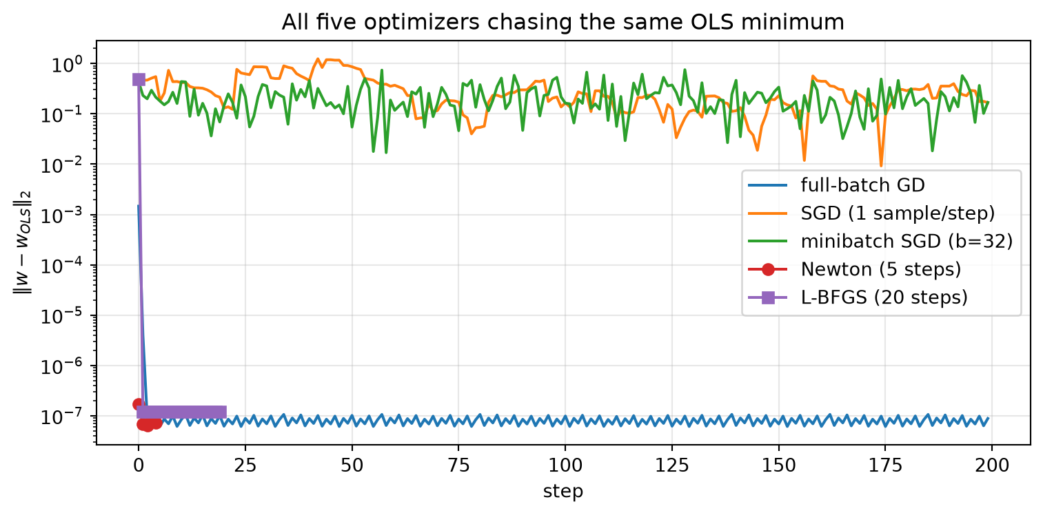

Reading the plot:

Newton lands in one step because the loss is a quadratic, so the local second-order Taylor model is exact globally.
L-BFGS also gets there fast, in ≤ 5 outer iterations.
Full-batch GD decays geometrically — the rate is set by the condition number of the Hessian. With standardisation that condition number is ~1, so GD is fast too.
SGD bounces around the minimum: the noise floor scales with \(\eta\).
Minibatch SGD is the practical compromise — averages out single-sample noise while still being one matrix-vector multiply per step.

(Forward-pointer: full optimization deep dive — momentum, Adam, conditioning — is MFML Unit 6.)

Block 3 — The loss function is a noise-model choice

So far we have used MSE because the homework used MSE. But MSE corresponds to the assumption that the residuals \(y - \hat y\) are Gaussian with constant variance. If they are not, MSE gives a biased estimator.

The fastest way to see this: contaminate the dataset with a few outliers (sensor failures, mis-recorded specimens) and refit with three different losses.

(see MFML §“loss as decision proxy”, §“MSE/MAE/Huber”; ML-PC §28 “bias-variance”)

# Build a contaminated copy: take the original 600 °C data and corrupt 3% of points.
torch.manual_seed(0)
X_clean = X.clone()
y_clean = y.clone()

n_outliers = max(1, int(0.03 * len(X_clean)))
outlier_idx = torch.randperm(len(X_clean))[:n_outliers]
y_dirty = y_clean.clone()
y_dirty[outlier_idx] += torch.empty(n_outliers).uniform_(300.0, 600.0)

# Use Adam for all three losses: it adapts per-parameter step sizes so a single
# `lr` works on the raw stress / strain scale (the design matrix is hopelessly
# ill-conditioned in raw units; see Block 1's "Why standardise?" sidebar).
# Adam is forward-pointed in MFML §"beyond vanilla SGD".
def fit_with_loss(loss_module, n_iters=2000, lr=3.0):
    torch.manual_seed(0)
    m = nn.Linear(1, 1)
    opt = torch.optim.Adam(m.parameters(), lr=lr)
    Xc = X_clean.unsqueeze(1)
    for _ in range(n_iters):
        opt.zero_grad()
        loss = loss_module(m(Xc).squeeze(1), y_dirty)
        loss.backward()
        opt.step()
    return m

m_mse   = fit_with_loss(nn.MSELoss())
# delta=10 sits just above the typical inlier residual scale (~5 MPa) and well
# below the outlier injections (300+ MPa). So inliers stay in the quadratic
# regime and outliers in the linear regime — exactly the split Huber is built
# to make. Picking delta is data-dependent: too small acts like MAE, too large
# acts like MSE.
m_huber = fit_with_loss(nn.HuberLoss(delta=10.0))
m_mae   = fit_with_loss(nn.L1Loss())

xs_grid = torch.linspace(X_clean.min(), X_clean.max(), 200).unsqueeze(1)
with torch.no_grad():
    yh_mse   = m_mse(xs_grid).squeeze().numpy()
    yh_huber = m_huber(xs_grid).squeeze().numpy()
    yh_mae   = m_mae(xs_grid).squeeze().numpy()

# Reference: OLS on the *clean* data — the "what would an outlier-free MSE give?" line.
A_c = torch.stack([X_clean, torch.ones_like(X_clean)], dim=1)
w_ref = torch.linalg.lstsq(A_c, y_clean.unsqueeze(1)).solution.squeeze()
yh_ref = (w_ref[0] * xs_grid.squeeze() + w_ref[1]).numpy()

print(f"slope (clean OLS):   {w_ref[0]:7.2f}")
print(f"slope (MSE on dirty):  {m_mse.weight.item():7.2f}   <- pulled UP by outliers")
print(f"slope (Huber on dirty):{m_huber.weight.item():7.2f}   <- much closer to clean OLS than MSE; still slightly biased")
print(f"slope (MAE on dirty):  {m_mae.weight.item():7.2f}   <- median, not mean — different story (see take-away)")

slope (clean OLS):    421.62
slope (MSE on dirty):   628.89   <- pulled UP by outliers
slope (Huber on dirty): 360.57   <- much closer to clean OLS than MSE; still slightly biased
slope (MAE on dirty):   115.33   <- median, not mean — different story (see take-away)

fig, ax = plt.subplots(1, 2, figsize=(11, 4))
ax[0].scatter(X_clean.numpy(), y_dirty.numpy(), s=10, alpha=0.5, label='dirty data')
ax[0].plot(xs_grid.numpy().squeeze(), yh_ref,   'k--', lw=1.5, label='OLS on CLEAN data')
ax[0].plot(xs_grid.numpy().squeeze(), yh_mse,   label='MSE')
ax[0].plot(xs_grid.numpy().squeeze(), yh_huber, label='Huber')
ax[0].plot(xs_grid.numpy().squeeze(), yh_mae,   label='MAE (L1)')
ax[0].set_xlabel('strain'); ax[0].set_ylabel('stress'); ax[0].legend(); ax[0].set_title('three losses, same dirty data')

# Residual histograms — clip the x-axis to the inlier range so the outlier tail
# doesn't squash everything into one bar at zero. The shifts among MSE / Huber /
# MAE are visible only in the inlier band.
with torch.no_grad():
    r_mse   = (y_dirty - m_mse(X_clean.unsqueeze(1)).squeeze(1)).numpy()
    r_huber = (y_dirty - m_huber(X_clean.unsqueeze(1)).squeeze(1)).numpy()
    r_mae   = (y_dirty - m_mae(X_clean.unsqueeze(1)).squeeze(1)).numpy()
inlier_bins = np.linspace(-25, 25, 50)
ax[1].hist(r_mse,   bins=inlier_bins, alpha=0.5, label='MSE residuals')
ax[1].hist(r_huber, bins=inlier_bins, alpha=0.5, label='Huber residuals')
ax[1].hist(r_mae,   bins=inlier_bins, alpha=0.5, label='MAE residuals')
ax[1].axvline(0, color='k', lw=0.5, alpha=0.5)
ax[1].set_xlim(-25, 25)
ax[1].set_xlabel('residual (MPa, inlier band)'); ax[1].set_ylabel('count')
ax[1].legend(); ax[1].set_title(f'residual distributions ({n_outliers} outlier residuals at ~+300..+500 not shown)')
plt.tight_layout(); plt.show()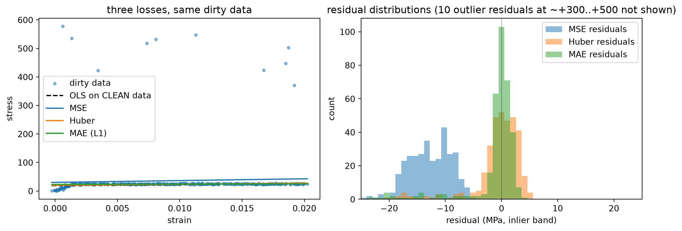

Reading the picture. Three regimes:

MSE drifts noticeably toward the outliers — because it is the negative log-likelihood of a Gaussian, and Gaussians have no heavy tail to absorb them. Each outlier contributes a quadratic penalty that the optimizer pays by tilting the line.
Huber stays close to “OLS on clean data” — the dashed line. Huber tells you “treat small residuals as squared, large residuals as absolute” — which is exactly what robust statistics has said since the 1960s. This is the right move when you trust most of your data and want one or two specimens to not dictate the fit.
MAE goes somewhere different on its own. L1 regression solves for the median residual, not the mean — and on a curved stress–strain plot the median line is dominated by the dense cloud of low-strain low-stress points, giving a much shallower slope. So MAE is “robust to outliers” and “robust to the curvature being wrong” — it solves a different problem from MSE.

Decision rule for the semester: plot the residuals. Heavy tails → drop MSE in favour of Huber. Want central tendency, not mean? Use MAE. Want the Gaussian assumption to actually hold? Use MSE — and check the residuals.

Block 4 — Basis functions: polynomial → Runge → cubic spline

nn.Linear(1, 1) cannot fit the post-yield work-hardening tail. Time for the linearity-in-parameters trick from MFML: replace strain \(x\) with a vector of basis functions \(\phi(x) = [\phi_0(x), \phi_1(x), \dots, \phi_{p-1}(x)]^\top\), then fit \(\hat y = w^\top \phi(x)\).

Two bases: 1. Polynomial: \(\phi_k(x) = x^k\). Easy to write, but high degrees suffer from Runge’s phenomenon — wild oscillations near data boundaries. 2. Cubic B-spline: piecewise cubics joined smoothly at knots. Locally flexible, globally well-behaved.

(see MFML §“linearity principle”, §“Runge’s phenomenon”, §“splines”)

def polynomial_basis(x, degree):
    """Returns the design matrix [1, x, x^2, ..., x^degree], shape (N, degree+1).

    NOTE: for `degree > ~6`, the caller must rescale `x` to roughly [-1, 1]
    first (see `to_unit` below) — otherwise high-degree columns underflow and
    the design matrix becomes numerically rank-deficient. The function space
    is unchanged by the rescaling.
    """
    cols = [torch.ones_like(x)]
    for k in range(1, degree + 1):
        cols.append(x ** k)
    return torch.stack(cols, dim=1)

def cubic_bspline_basis(x_np, n_knots):
    """Returns a clamped cubic B-spline design matrix, shape (N, n_basis_functions).

    Uses scipy for the basis construction; the regression itself stays in torch.
    """
    k = 3   # cubic
    knots_inner = np.linspace(x_np.min(), x_np.max(), n_knots)[1:-1]
    knots = np.concatenate(([x_np.min()] * (k + 1), knots_inner, [x_np.max()] * (k + 1)))
    n_basis = len(knots) - k - 1
    cols = []
    for j in range(n_basis):
        c = np.zeros(n_basis)
        c[j] = 1.0
        spline = BSpline(knots, c, k, extrapolate=False)
        cols.append(np.nan_to_num(spline(x_np)))
    return torch.tensor(np.stack(cols, axis=1), dtype=torch.float32)

def fit_basis(Phi, y):
    """Closed-form least squares via SVD (`torch.linalg.lstsq`).

    Equivalent to `(Phi^T Phi)^-1 Phi^T y` when Phi has full column rank,
    but uses the more stable SVD path so it gracefully handles rank-deficient
    Phi (e.g. high-degree polynomial bases on ill-conditioned data).
    """
    return torch.linalg.lstsq(Phi, y.unsqueeze(1)).solution.squeeze()

# Sort once for clean line plots.
order = torch.argsort(X)
X_sorted = X[order]
y_sorted = y[order]
xs_grid = torch.linspace(X_sorted.min(), X_sorted.max(), 400)

# Polynomial bases need x rescaled to ~[-1, 1] for numerical conditioning.
# Raw strain is ~1e-2, so x^15 underflows to ~1e-30 and the design matrix is
# numerically rank-deficient. The fit becomes a constant and you would not
# see Runge's phenomenon at all. Mapping to [-1, 1] preserves the polynomial
# function space (degree-d in (x-a)/b is still degree-d in x) -- it only
# moves the basis to a regime where double precision can represent it.
x_min, x_max = float(X_sorted.min()), float(X_sorted.max())
def to_unit(x):
    return 2.0 * (x - x_min) / (x_max - x_min) - 1.0

degrees   = [1, 5, 15]
n_knots_s = [4, 8, 16]

fig, ax = plt.subplots(2, 3, figsize=(13, 7), sharey=True)

for j, d in enumerate(degrees):
    Phi      = polynomial_basis(to_unit(X_sorted), d)
    Phi_grid = polynomial_basis(to_unit(xs_grid),  d)
    w        = fit_basis(Phi, y_sorted)
    yhat     = (Phi_grid @ w).numpy()
    ax[0, j].scatter(X_sorted.numpy(), y_sorted.numpy(), s=8, alpha=0.5)
    ax[0, j].plot(xs_grid.numpy(), yhat, 'r-', lw=2)
    ax[0, j].set_title(f"polynomial degree {d}")
    ax[0, j].set_xlabel("strain"); ax[0, 0].set_ylabel("stress")

for j, n in enumerate(n_knots_s):
    Phi      = cubic_bspline_basis(X_sorted.numpy(), n)
    Phi_grid = cubic_bspline_basis(xs_grid.numpy(),  n)
    w        = fit_basis(Phi, y_sorted)
    yhat     = (Phi_grid @ w).numpy()
    ax[1, j].scatter(X_sorted.numpy(), y_sorted.numpy(), s=8, alpha=0.5)
    ax[1, j].plot(xs_grid.numpy(), yhat, 'g-', lw=2)
    ax[1, j].set_title(f"cubic B-spline, {n} knots")
    ax[1, j].set_xlabel("strain"); ax[1, 0].set_ylabel("stress")

plt.suptitle("Polynomial bases (top) wiggle at high degree; spline bases (bottom) stay sane", y=1.02)
plt.tight_layout(); plt.show()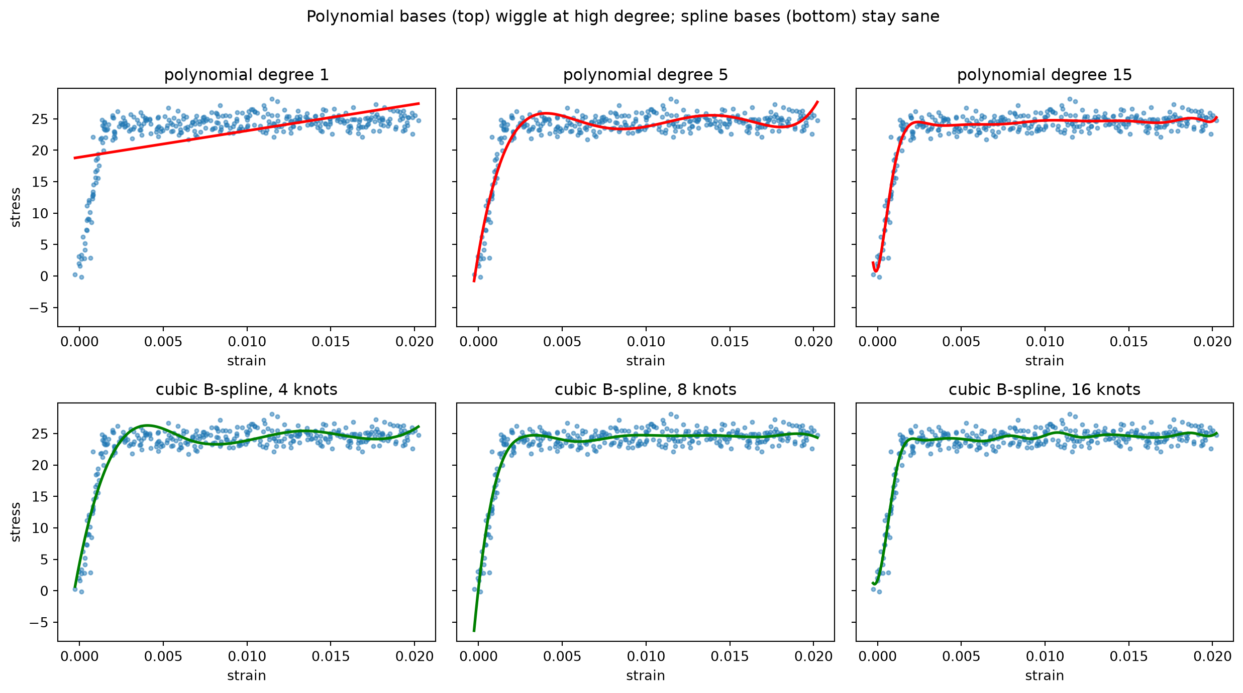

Reading the picture. A polynomial of degree 15 over-fits the noise and develops the Runge oscillation at the boundaries. A cubic spline with 16 knots uses about the same number of parameters but stays locally smooth — because each knot only influences its neighbourhood, the model can be flexible where the data needs it and rigid elsewhere.

Take-away: “more parameters” is a bad summary of model capacity. Where the parameters can flex matters more.

Block 5 — Three flavours of leakage

Block 4 gave us a great fit on 600 °C data. Now we ask the harder question: does that fit say anything about a new test specimen? The answer depends on how we split the data.

We will combine all three temperatures (0, 400, 600 °C) into one dataset with strain and temperature as features. Then evaluate the same spline regressor under three splits — each leaky in exactly one way — and compare to the honest split.

(see ML-PC §31–37 “holdout / K-fold / leakage”)

def make_combined_dataset():
    Xs, ys, T_groups = [], [], []
    for T in (0, 400, 600):
        ds = TensileTestDataset(temperature=T)
        strain = ds.X.squeeze(1).numpy()
        stress = ds.y.numpy()
        Xs.append(np.column_stack([strain, np.full_like(strain, T)]))
        ys.append(stress)
        T_groups.append(np.full_like(strain, T))
    X = np.vstack(Xs)
    y = np.concatenate(ys)
    g = np.concatenate(T_groups).astype(np.int64)
    return X, y, g

X_all_np, y_all_np, group_all = make_combined_dataset()
print(f"combined dataset: N={X_all_np.shape[0]}  D={X_all_np.shape[1]}  groups={set(group_all.tolist())}")


def fit_spline_2d(X_train, y_train, X_test, y_test, n_knots=8):
    """Fit a spline-in-strain * linear-in-temperature model. Returns test-R^2."""
    # Build the design matrix: spline on strain (col 0), interacted linearly with temperature (col 1).
    strain_train, temp_train = X_train[:, 0], X_train[:, 1]
    strain_test,  temp_test  = X_test[:,  0], X_test[:,  1]
    Phi_strain_train = cubic_bspline_basis(strain_train, n_knots)
    Phi_strain_test  = cubic_bspline_basis(strain_test,  n_knots)
    # Stack: [spline cols] + [spline cols * temperature].
    T_tr = torch.tensor(temp_train, dtype=torch.float32).unsqueeze(1)
    T_te = torch.tensor(temp_test,  dtype=torch.float32).unsqueeze(1)
    Phi_tr = torch.cat([Phi_strain_train, Phi_strain_train * T_tr], dim=1)
    Phi_te = torch.cat([Phi_strain_test,  Phi_strain_test  * T_te], dim=1)
    y_tr_t = torch.tensor(y_train, dtype=torch.float32)
    y_te_t = torch.tensor(y_test,  dtype=torch.float32)
    w = torch.linalg.lstsq(Phi_tr, y_tr_t.unsqueeze(1)).solution.squeeze()
    yhat = Phi_te @ w
    ss_res = ((y_te_t - yhat) ** 2).sum().item()
    ss_tot = ((y_te_t - y_te_t.mean()) ** 2).sum().item()
    return 1.0 - ss_res / max(ss_tot, 1e-12)

combined dataset: N=1050  D=2  groups={0, 600, 400}

5a — Pre-processing leakage (standardise before splitting)

rng = np.random.default_rng(0)

def split_random(X, y, frac_train=0.7):
    n = X.shape[0]
    perm = rng.permutation(n)
    cut = int(frac_train * n)
    return X[perm[:cut]], X[perm[cut:]], y[perm[:cut]], y[perm[cut:]]

# Honest: standardise INSIDE the train fold, then apply the same transform to test.
X_tr, X_te, y_tr, y_te = split_random(X_all_np, y_all_np)
mu, sd = X_tr.mean(axis=0), X_tr.std(axis=0)
X_tr_h = (X_tr - mu) / sd
X_te_h = (X_te - mu) / sd
r2_honest_pp = fit_spline_2d(X_tr_h, y_tr, X_te_h, y_te)

# Leaky: standardise the WHOLE dataset first, then split. Test stats bleed into train.
mu_all, sd_all = X_all_np.mean(axis=0), X_all_np.std(axis=0)
X_full_scaled = (X_all_np - mu_all) / sd_all
rng = np.random.default_rng(0)  # reset so the row indices match
X_tr_l, X_te_l, y_tr_l, y_te_l = split_random(X_full_scaled, y_all_np)
r2_leaky_pp = fit_spline_2d(X_tr_l, y_tr_l, X_te_l, y_te_l)

print(f"5a pre-processing  | honest R^2 = {r2_honest_pp:.3f}    leaky R^2 = {r2_leaky_pp:.3f}    gap = {r2_leaky_pp - r2_honest_pp:+.3f}")

5a pre-processing  | honest R^2 = 0.888    leaky R^2 = 0.888    gap = -0.000

5b — Group leakage (random K-fold across temperatures)

def random_kfold(X, y, k=5):
    n = X.shape[0]
    perm = np.random.default_rng(0).permutation(n)
    folds = np.array_split(perm, k)
    scores = []
    for i in range(k):
        te = folds[i]
        tr = np.concatenate([folds[j] for j in range(k) if j != i])
        scores.append(fit_spline_2d(X[tr], y[tr], X[te], y[te]))
    return float(np.mean(scores))

def group_kfold(X, y, groups, k=3):
    """Leave-one-group-out — here k=3 because we have 3 temperatures."""
    unique_g = np.unique(groups)
    scores = []
    for g in unique_g:
        te_mask = groups == g
        scores.append(fit_spline_2d(X[~te_mask], y[~te_mask], X[te_mask], y[te_mask]))
    return float(np.mean(scores))

r2_random_cv = random_kfold(X_all_np, y_all_np, k=5)
r2_group_cv  = group_kfold(X_all_np, y_all_np, group_all)
print(f"5b group           | random K-fold R^2 = {r2_random_cv:.3f}   group K-fold R^2 = {r2_group_cv:.3f}   gap = {r2_random_cv - r2_group_cv:+.3f}")

5b group           | random K-fold R^2 = 0.888   group K-fold R^2 = -4.160   gap = +5.048

5c — Temporal leakage (predicting the past from the future)

def split_temporal(X, y, groups, train_late=True):
    """Within each group, take the late half as train (or test, if not train_late)."""
    tr_idx, te_idx = [], []
    for g in np.unique(groups):
        in_g = np.where(groups == g)[0]
        in_g_sorted = in_g[np.argsort(X[in_g, 0])]   # sort by strain == time within a tensile test
        cut = len(in_g_sorted) // 2
        if train_late:
            tr_idx.extend(in_g_sorted[cut:].tolist())
            te_idx.extend(in_g_sorted[:cut].tolist())
        else:
            tr_idx.extend(in_g_sorted[:cut].tolist())
            te_idx.extend(in_g_sorted[cut:].tolist())
    tr_idx = np.array(tr_idx); te_idx = np.array(te_idx)
    return X[tr_idx], X[te_idx], y[tr_idx], y[te_idx]

# Honest temporal split: train on early time -> predict late time (the realistic
# scenario for a process-monitoring model).
X_tr, X_te, y_tr, y_te = split_temporal(X_all_np, y_all_np, group_all, train_late=False)
r2_honest_t = fit_spline_2d(X_tr, y_tr, X_te, y_te)

# Leaky: train on LATE -> predict EARLY (predicting the past from the future).
X_tr, X_te, y_tr, y_te = split_temporal(X_all_np, y_all_np, group_all, train_late=True)
r2_leaky_t  = fit_spline_2d(X_tr, y_tr, X_te, y_te)

print(f"5c temporal        | honest (train→future) R^2 = {r2_honest_t:.3f}   leaky (train←future) R^2 = {r2_leaky_t:.3f}   gap = {r2_leaky_t - r2_honest_t:+.3f}")

5c temporal        | honest (train→future) R^2 = -0.051   leaky (train←future) R^2 = -0.032   gap = +0.019

# Bar chart: visual summary of all three demos. Clip the y-axis to [-1, 1.05]
# so the brutal group-leakage R² (around -4) doesn't crush the visual; the
# negative bar is annotated so students still see how bad it is.
labels = ['5a pre-proc', '5b group', '5c temporal']
honest = [r2_honest_pp, r2_group_cv,  r2_honest_t]
leaky  = [r2_leaky_pp,  r2_random_cv, r2_leaky_t]
xpos = np.arange(len(labels))

plt.figure(figsize=(8, 4))
plt.bar(xpos - 0.2, honest, width=0.4, label='honest')
plt.bar(xpos + 0.2, leaky,  width=0.4, label='leaky')
plt.xticks(xpos, labels); plt.ylabel(r'$R^2$ on test')
plt.title("Three flavours of leakage — same model, same data, different verdicts")
plt.axhline(0, color='k', lw=0.5)
plt.ylim(-1.0, 1.05)
# Annotate any clipped bars with their actual value.
for i, (h_val, l_val) in enumerate(zip(honest, leaky)):
    if h_val < -1.0:
        plt.text(i - 0.2, -0.95, f'{h_val:.2f}', ha='center', va='bottom', fontsize=8, color='white')
    if l_val < -1.0:
        plt.text(i + 0.2, -0.95, f'{l_val:.2f}', ha='center', va='bottom', fontsize=8, color='white')
plt.legend(); plt.grid(axis='y', alpha=0.3); plt.tight_layout(); plt.show()

max_gap = max(abs(l - h) for l, h in zip(leaky, honest))
print(f"\nlargest leaky-vs-honest R^2 gap: {max_gap:.3f}")
assert max_gap >= 0.10, (
    f"acceptance criterion failed: largest gap is {max_gap:.3f} < 0.10. "
    "Tune n_knots or split fractions to widen the gap before shipping."
)


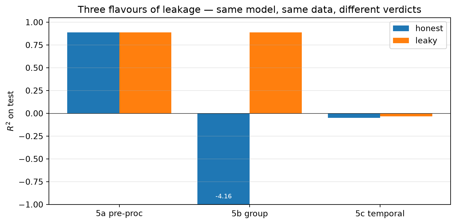
largest leaky-vs-honest R^2 gap: 5.048

The take-away. Same model, same data, three different verdicts.

Not all leakage flavours bite the same model equally. Reading the bar chart:

5a (pre-processing) — for our linear-in-parameters spline, simple (x - mean) / std is absorbed by the weights: feature scaling is just an affine transform that the model can undo. So the gap is essentially zero. The classic preprocessing leak that DOES bite linear models is non-affine — PCA-fit on full data, percentile-clipping on full data, mean-imputation, or feature selection that uses the test set. The lesson stands: any preprocessing step that summarises the test fold leaks; whether your model notices depends on the model.
5b (group) — brutal. Random K-fold across temperatures gives R² ≈ 0.89; honest leave-one-temperature-out gives R² strongly negative (~-4) because the model has never seen the held-out temperature and can’t extrapolate. Every materials-science train/test split should ask: what’s the group variable my model is silently learning to memorise? For us today it’s temperature; in your work it might be specimen-id, instrument-batch, or even date-of-experiment.
5c (temporal) — both directions are bad here, with a small (~0.02) edge for the leaky direction. The bimodal stress–strain curve (elastic regime then plateau) means neither half of the data extrapolates to the other — the model needs to see both regimes. Temporal splits that work well live in the supplementary ML-PC time-series deck; the lesson here is that even an “honest” temporal split can have R² well below random K-fold.

Defensive habit: before reporting a CV score, ask: 1. Did the test fold see any preprocessing statistics from the train fold? (5a) 2. Does each test row have a near-identical sibling in the train fold? (5b) 3. Does the train fold contain information that postdates the test fold? (5c)

If yes to any of them, your validation is leaking and your test-R² is fiction.

Block 6 — Student exercises (~35 min)

Attempt Exercises 1–3 in order. Exercise 4 is a stretch goal.

Each exercise is annotated with the lecture learning outcome it tests, so you can self-check what you understood.

Exercise 1 — Outlier surgery, loss choice

Tests MFML LO4: pick the loss that matches the noise model.

A contaminated tensile-test dataset is provided as X_clean, y_dirty from Block 3 — keep using those variables.

Tasks:

Fit three models with nn.MSELoss, nn.HuberLoss(delta=...) (you choose the delta), and nn.L1Loss. Use the same training-loop scaffold as Block 3.
Plot residual histograms for each model.
Pick the loss whose residual histogram looks closest to a zero-mean, light-tailed distribution. Justify your pick in 2 sentences.
State the value of delta you used for Huber and explain how you chose it.

# Your code for Exercise 1 goes here.
# m_mse_ex1 = ...
# m_huber_ex1 = ...
# m_mae_ex1 = ...

Exercise 2 — Roll your own GroupKFold

Tests ML-PC LO: leakage-aware validation.

Tasks:

Write a function my_group_kfold(groups) that yields a sequence of (train_idx, test_idx) pairs, where each fold holds out exactly one group. Cap it at ≤ 20 lines.
Apply it to the combined-temperature TensileTest data with temperature as the group; report the mean test-R² and compare against sklearn.model_selection.GroupKFold.
Also report a plain random K-fold R² (k=5). The gap is your group-leakage measurement on this dataset.

# Your code for Exercise 2 goes here.
# def my_group_kfold(groups):
#     ...
#
# from sklearn.model_selection import GroupKFold  # for verification only
# ...

Exercise 3 — Spline vs polynomial bias-variance

Tests MFML LO6: recognise Runge / choose between bases.

Tasks:

Use the 600 °C data only. Hold out the last 20% of (sorted-by-strain) points as a validation set.
For polynomial degree \(d \in \{1, 2, 3, 5, 8, 12, 15\}\), fit on the train half and record train-MSE and val-MSE.
Repeat for cubic B-spline with n_knots ∈ {3, 4, 6, 8, 12, 16}.
Plot both train-MSE and val-MSE on log-y, side by side for the two bases.
Annotate on each plot: which region is bias-dominated, which is variance-dominated, and which is the sweet spot.

# Your code for Exercise 3 goes here.
# degrees = [1, 2, 3, 5, 8, 12, 15]
# n_knots = [3, 4, 6, 8, 12, 16]
# ...

Exercise 4 (stretch) — Leakage detective

Tests ML-PC LO: leakage diagnosis on unseen data.

Load data/week3_mystery.npz — it contains three pre-built train/test splits named split_A, split_B, split_C. Each is leaky in exactly one of the three ways from Block 5 (preprocessing / group / temporal). Your job is to diagnose which is which.

Tasks:

For each split, fit any reasonable model and report train-R² and test-R².
For each split, write down ONE diagnostic test that distinguishes its leakage type from the other two. Examples: “I’ll plot the per-row temperature of train vs test”, or “I’ll re-fit after re-shuffling and see whether scores change.”
Run your diagnostics and write your guess for each split.
Only after writing your guess, open data/week3_mystery_solutions.txt and confirm.

# Your code for Exercise 4 (stretch) goes here.
# import numpy as np
# z = np.load('../data/week3_mystery.npz')
# for letter in ('A', 'B', 'C'):
#     X_tr = z[f'split_{letter}_X_train']
#     X_te = z[f'split_{letter}_X_test']
#     y_tr = z[f'split_{letter}_y_train']
#     y_te = z[f'split_{letter}_y_test']
#     ...

Wrap-up: the red thread, restated

Today you saw the same data behave like a great success or a quiet failure depending on two choices that have nothing to do with the model architecture:

Which loss did you minimise? Pick the one whose negative log-likelihood matches your noise model. MSE for Gaussian, Huber for “Gaussian with rare outliers”, Poisson NLL for low-count data (week 2), MAE for “I really do want to minimise the median residual.”
Which split did you evaluate on? Random row-shuffle is a dangerous default. Ask: is preprocessing fitted on the train fold only? Are correlated rows (same specimen, same temperature, same instrument run) kept together? Does train-time precede test-time?

Forward-pointers (already on the syllabus):

MFML Unit 6 — full first-order optimization (momentum, Adam, conditioning).
MFML Unit 7 — full Bayesian / MAP picture; the loss-as-NLL framing made formal.
ML-PC week 5 — image segmentation metrics (Dice, IoU) — the categorical counterpart to today’s MSE/MAE story.
ML-PC Unit 7 supplementary time-series deck — temporal splits are the default there.
MFML Unit 7 — Bayesian regression / conformal prediction; today’s L2-regularisation already secretly put a Gaussian prior on the weights (MAP interpretation).
MFML Unit 12 — Gaussian processes, MC dropout, active learning — posterior-driven uncertainty for materials discovery.

Things we deliberately did not cover today (each has a home elsewhere):

GLM / exponential family / IRLS — see the GLM materials when they appear later.
Probabilistic labels / inter-annotator variance — comes back in MFML Unit 12.