MFML Unit 4: From dense layers and activations to convolution — why CNNs are the right inductive bias for image-like data.
ML-PC Unit 4: From classical metrics to learned representations — why the encoding of microstructure data often dominates the model.
Red thread:On the same Ising classification task we will train three models — a flat MLP, a tiny CNN, and a linear classifier on a single hand-crafted scalar (mean magnetisation). The three answers will not agree. Reading off which one wins, and why, is the entire point of today’s class.
Pre-flight check. This notebook assumes you have run notebooks/week4_homework.py. Block 1 picks up directly from your Part C flat-MLP baseline, and Block 2 checks the Part D parameter-count answer.
Agenda (90 min)
Block
Min
Topic
1
~6
Recap from homework — flat MLP baseline on Ising-light
2
~10
The image problem — parameter explosion at 64×64
3
~10
Roll-your-own convolution with F.conv2d + equivariance demo
4
~12
A tiny CNN — trace tensor shapes; train; compare to MLP
# Standard imports. Same idiom as weeks 2 and 3: explicit seeds, no hidden state.import numpy as npimport torchimport torch.nn as nnimport torch.nn.functional as Ffrom torch.utils.data import DataLoader, random_split, Subsetimport matplotlib.pyplot as pltfrom ai4mat.datasets import IsingDatasetnp.random.seed(0)torch.manual_seed(0)
<torch._C.Generator at 0x7f5c98156ff0>
Helpers used by every block
We reuse one training loop and one evaluator across blocks 1, 4, 6 so the only thing that changes between experiments is the model and the representation. That makes the comparisons honest.
def evaluate(model, loader): model.eval() correct = total =0with torch.no_grad():for x, y_ in loader: correct += (model(x).argmax(dim=1) == y_).sum().item() total += y_.numel()return correct / totaldef train(model, train_loader, val_loader, epochs=10, lr=1e-3, log=True):"""Standard supervised loop. Returns list of per-epoch val accuracies.""" opt = torch.optim.Adam(model.parameters(), lr=lr) loss_fn = nn.CrossEntropyLoss() val_hist = []for epoch inrange(epochs): model.train()for x, y_ in train_loader: opt.zero_grad() loss = loss_fn(model(x), y_) loss.backward() opt.step() v = evaluate(model, val_loader) val_hist.append(v)if log:print(f" epoch {epoch +1:2d} val acc = {v *100:5.2f}%")return val_histdef n_params(model) ->int:returnsum(p.numel() for p in model.parameters() if p.requires_grad)
Block 1 — Recap from homework: flat MLP on Ising-light
Reproduce your homework Part C in 10 lines and lock in the baseline numbers. Everything in the rest of the lecture is compared against this.
(see MFML §“Dense networks learn features”; ML-PC §“Image as Tensor”)
# A flat-MLP baseline: same shape as the homework's Part C, restated here# verbatim so this notebook is self-contained.torch.manual_seed(0)flat_mlp = nn.Sequential( nn.Flatten(), nn.Linear(16*16, 64), nn.ReLU(), nn.Linear(64, 32), nn.ReLU(), nn.Linear(32, 2),)print(f"flat MLP params: {n_params(flat_mlp):,}")print("training flat MLP on Ising-light...")mlp_hist = train(flat_mlp, train_loader, val_loader, epochs=10, log=True)acc_flat_mlp = mlp_hist[-1]
flat MLP params: 18,594
training flat MLP on Ising-light...
  epoch  1   val acc = 69.50%
  epoch  2   val acc = 75.40%
  epoch  3   val acc = 75.00%
  epoch  4   val acc = 87.30%
  epoch  5   val acc = 87.90%
  epoch  6   val acc = 89.60%
  epoch  7   val acc = 89.70%
  epoch  8   val acc = 90.50%
  epoch  9   val acc = 90.60%
  epoch 10   val acc = 91.70%
Lock in this number (final val accuracy of the flat MLP). Every model in blocks 4 and 6 has to beat it — or explain why it cannot.
Block 2 — The image problem: parameter explosion
Your homework Part D worked out the parameter count of a flat MLP on 64×64 images analytically. Here we (a) verify the formula, and (b) make the trainability problem concrete by counting both parameters and bytes.
(see MFML §“The dense image problem”, §“Parameter economy”)
     image | MLP first layer |  CNN feature extractor
--------------------------------------------------------
  16 x 16  |          65,792 |                  5,888
  32 x 32  |         262,400 |                  5,888
  64 x 64  |       1,048,832 |                  5,888
 128 x 128 |       4,194,560 |                  5,888
 256 x 256 |      16,777,472 |                  5,888
Read this table aloud. The MLP first-layer count grows quadratically with the image side — a 256² image already burns 16 million weights just for the input projection. The CNN feature extractor is constant in image size: it only depends on channel counts and kernel size, not on H × W.
That difference is the architectural argument for convolution. Locality + weight sharing trade representational generality for parameter efficiency, and the trade is overwhelmingly worth it for image-shaped data.
# Memory-cost sanity check: float32 = 4 bytes per parameter.n_mlp_64 = mlp_first_layer(64*64, 256)print(f"flat MLP first-layer storage at 64x64 hidden=256: "f"{n_mlp_64 *4/1e6:.2f} MB just for the weight matrix")
flat MLP first-layer storage at 64x64 hidden=256: 4.20 MB just for the weight matrix
Block 3 — Roll-your-own convolution with F.conv2d
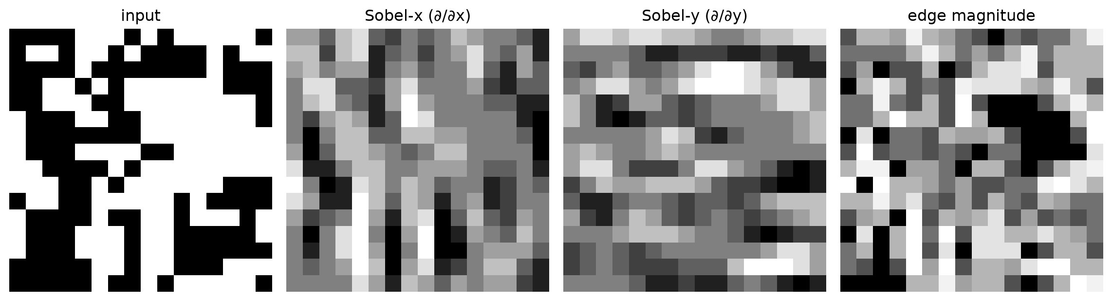
Before we let nn.Conv2d learn its kernels, we hand-place a Sobel-like edge detector and apply it with the bare functional API. Two observations:
A convolution is just a sliding inner product with a small kernel — nothing magical.
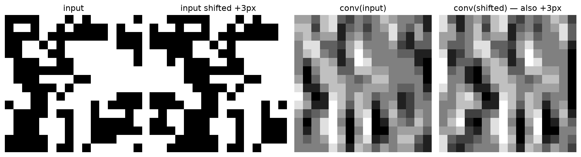
The same kernel applied at every position gives translation equivariance: shift the input, and the output shifts the same amount. This is the property that lets one filter recognise the same feature anywhere in the image.
(see MFML §“Weight sharing gives convolution”, §“Cross-correlation: the operation used in CNNs”, §“Sliding-window view”, §“A hand-computable filter”, §“Invariance vs equivariance”)
# Pick one Ising image to play with.img = ds_light.X[0:1] # shape (1, 1, 16, 16); a batch of 1 with 1 channelprint(f"image shape: {tuple(img.shape)}")# A 3x3 Sobel-x kernel detects vertical edges; rotate 90 degrees for Sobel-y.kx = torch.tensor([[[[-1, 0, 1], [-2, 0, 2], [-1, 0, 1]]]], dtype=torch.float32) # shape (1, 1, 3, 3)ky = kx.transpose(2, 3)
# Equivariance demo: shift the input by 3 pixels right; the output shifts the# same way. Translation in -> translation out.shifted = torch.roll(img, shifts=3, dims=3)edge_shifted = F.conv2d(shifted, kx, padding=1)fig, axes = plt.subplots(1, 4, figsize=(12, 3.2))for ax, im, title inzip( axes, [img[0, 0], shifted[0, 0], edge_x[0, 0], edge_shifted[0, 0]], ["input", "input shifted +3px", "conv(input)", "conv(shifted) — also +3px"],): ax.imshow(im.numpy(), cmap="gray"); ax.set_title(title); ax.axis("off")plt.tight_layout(); plt.show()
Take-home. A CNN doesn’t invent the property “the same feature at every location should give the same response” — convolution enforces it. That’s what the MLP cannot do without paying the parameter cost of relearning the same feature at every pixel.
Block 4 — A tiny CNN, end to end
Build a Conv → ReLU → Pool → Conv → ReLU → Pool → Linear network. Trace the tensor shapes through every layer (the shape checklist from the lecture). Train. Read off val accuracy and parameter count, and compare to the flat MLP from Block 1.
(see MFML §“Shape checklist”, §“Padding”, §“Stride”, §“Pooling”, §“From layers to blocks”, §“LeNet”)
class TinyCNN(nn.Module):def__init__(self):super().__init__()self.conv1 = nn.Conv2d(1, 8, kernel_size=3, padding=1) # (B,1,16,16) -> (B,8,16,16)self.conv2 = nn.Conv2d(8, 16, kernel_size=3, padding=1) # (B,8, 8, 8) -> (B,16, 8, 8)self.pool = nn.MaxPool2d(2) # halves H and Wself.head = nn.Linear(16*4*4, 2) # final spatial 4x4def forward(self, x): x = F.relu(self.conv1(x)) # (B, 8, 16, 16) x =self.pool(x) # (B, 8, 8, 8) x = F.relu(self.conv2(x)) # (B, 16, 8, 8) x =self.pool(x) # (B, 16, 4, 4) x = x.flatten(1) # (B, 256)returnself.head(x) # (B, 2)torch.manual_seed(0)cnn = TinyCNN()print(cnn)print(f"tiny CNN params: {n_params(cnn):,} (flat MLP was {n_params(flat_mlp):,})")
training tiny CNN on Ising-light...
  epoch  1   val acc = 89.70%
  epoch  2   val acc = 95.80%
  epoch  3   val acc = 96.40%
  epoch  4   val acc = 94.30%
  epoch  5   val acc = 96.40%
  epoch  6   val acc = 95.00%
  epoch  7   val acc = 94.60%
  epoch  8   val acc = 96.40%
  epoch  9   val acc = 96.50%
  epoch 10   val acc = 96.10%
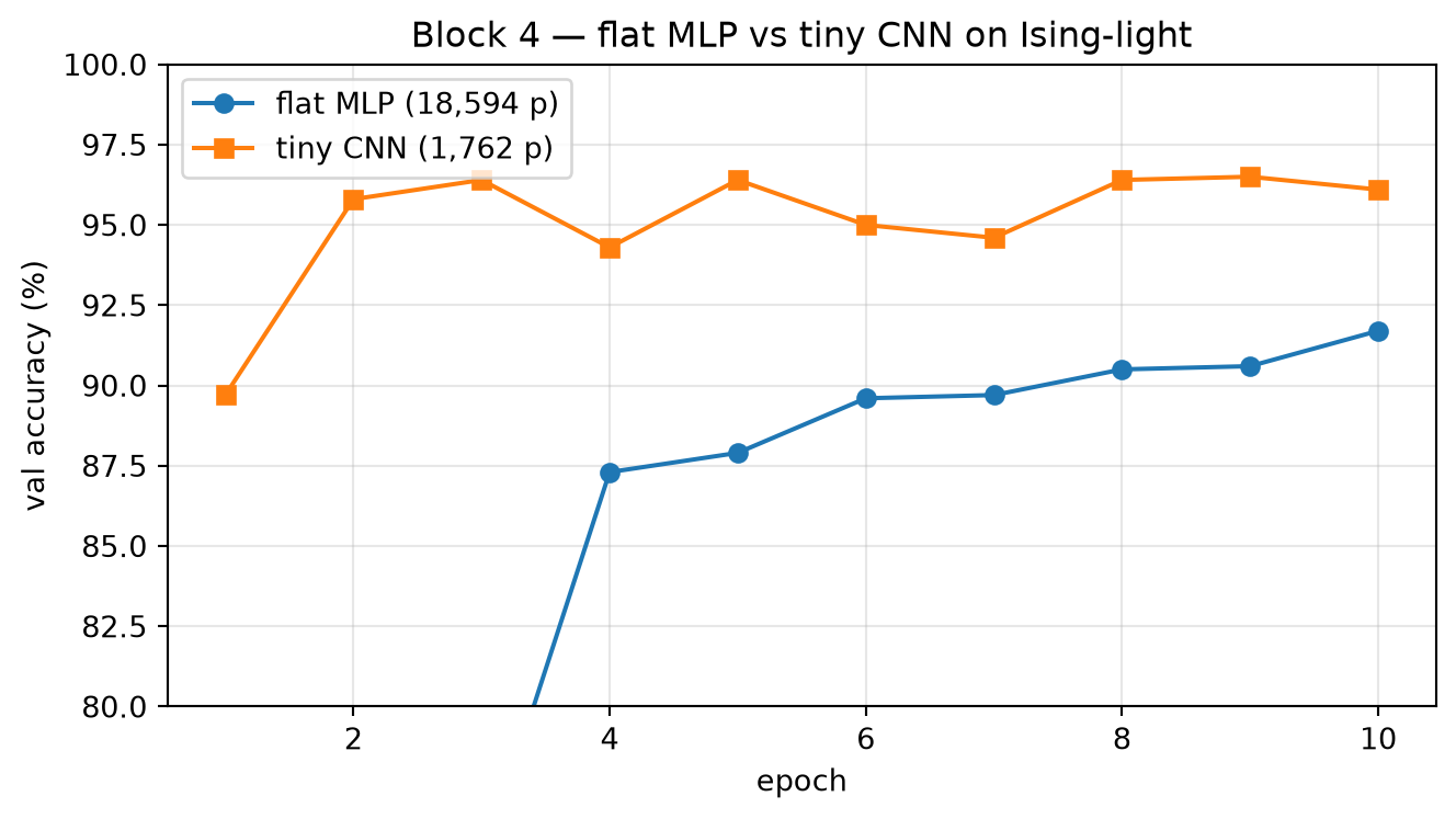
# Side-by-side comparison.fig, ax = plt.subplots(figsize=(7, 4))ax.plot(range(1, 11), [v *100for v in mlp_hist], "o-", label=f"flat MLP ({n_params(flat_mlp):,} p)")ax.plot(range(1, 11), [v *100for v in cnn_hist], "s-", label=f"tiny CNN ({n_params(cnn):,} p)")ax.set_xlabel("epoch"); ax.set_ylabel("val accuracy (%)")ax.set_title("Block 4 — flat MLP vs tiny CNN on Ising-light")ax.legend(); ax.grid(True, alpha=0.3); ax.set_ylim(80, 100)plt.tight_layout(); plt.show()print(f"\nflat MLP final acc : {acc_flat_mlp *100:.2f}% ({n_params(flat_mlp):>6,} params)")print(f"tiny CNN final acc : {acc_cnn *100:.2f}% ({n_params(cnn):>6,} params)")
flat MLP final acc : 91.70%   (18,594 params)
tiny CNN final acc : 96.10%   ( 1,762 params)
What you should see. The tiny CNN reaches comparable or better accuracy than the flat MLP with substantially fewer parameters. Same data, same loss, same optimizer — only the inductive bias changed. That is the convolution argument, demonstrated at desk scale.
Block 5 — Receptive fields: what does each filter see?
A receptive field is the region of the input that influences a single activation. For a 3×3 kernel, layer-1 RF = 3×3. After a stride-2 pool, the next 3×3 conv sees a 7×7 patch in the original image. By stacking blocks the RF grows quickly without adding many parameters — that’s how CNNs build a hierarchy of features.
(see MFML §“Receptive fields”, §“Hierarchy of learned features”)
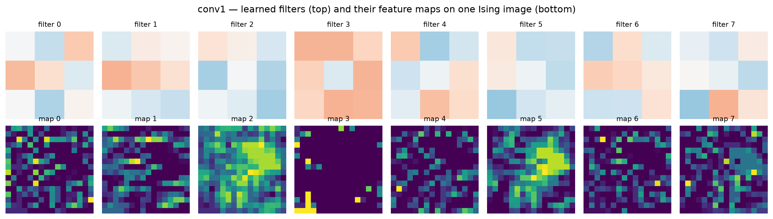
# Visualise the 8 learned filters of conv1 and a sample of feature maps.with torch.no_grad(): w1 = cnn.conv1.weight.detach().clone() # (8, 1, 3, 3) feat = F.relu(cnn.conv1(ds_light.X[:1])) # (1, 8, 16, 16)fig, axes = plt.subplots(2, 8, figsize=(14, 4))for i inrange(8): axes[0, i].imshow(w1[i, 0].numpy(), cmap="RdBu", vmin=-1, vmax=1) axes[0, i].set_title(f"filter {i}", fontsize=9); axes[0, i].axis("off") axes[1, i].imshow(feat[0, i].numpy(), cmap="viridis") axes[1, i].set_title(f"map {i}", fontsize=9); axes[1, i].axis("off")fig.suptitle("conv1 — learned filters (top) and their feature maps on one Ising image (bottom)")plt.tight_layout(); plt.show()
# Compute receptive-field size for the network analytically.# Formula: rf_l = rf_{l-1} + (k_l - 1) * stride_so_far# Each MaxPool(2) doubles the stride.def receptive_field(layers):"""layers: list of (kernel, stride). Returns RF in input pixels.""" rf, stride_so_far =1, 1for k, s in layers: rf += (k -1) * stride_so_far stride_so_far *= sreturn rf, stride_so_farlayers = [(3, 1), (2, 2), (3, 1), (2, 2)] # conv1, pool, conv2, poolrf, stride = receptive_field(layers)print(f"final-layer activation receptive field: {rf} x {rf} input pixels "f"(input is 16x16, so each unit sees ~{100* rf * rf /256:.0f}% of the image)")
final-layer activation receptive field: 10 x 10 input pixels (input is 16x16, so each unit sees ~39% of the image)
Take-home. Learned filters look like local patterns — edges, blobs, alignments — not like global pixel-by-pixel templates. That is the representation a CNN learns for free from data + the locality bias.
Block 6 — Representation showdown
Three pipelines on the same Ising labels:
Raw pixels → flat MLP (Block 1).
Raw pixels → tiny CNN (Block 4).
Hand-crafted scalar (mean magnetisation per image) → linear classifier.
Recall that the Ising label is “above or below the Curie temperature” — i.e., whether the system is paramagnetic or ferromagnetic. The order parameter that physicists defined for this system is the magnitude of the mean magnetisation. A linear classifier on that one number is the smallest possible model that uses the right physics.
(see ML-PC §“The Information Bottleneck”, §“Hero Result — Steel Phase Classification”, §“The Paradigm Shift”, §“Encoding Decision Rule”)
# Compute mean magnetisation per image. Ising images are stored in [0, 1];# the original spins are {-1, +1}. Recover the spin field, then average per image.spins = (ds_light.X *2-1).squeeze(1) # (N, 16, 16) in {-1, +1}mean_M = spins.mean(dim=(1, 2)).abs().unsqueeze(1) # (N, 1) -- |<m>| order parameter# Sanity check: high-T should average toward 0; low-T toward 1.for k in [0, 1]: m = mean_M[ds_light.y == k].mean().item()print(f"label {k} ({'high-T'if k ==0else'low-T'}): mean |M| = {m:.3f}")
label 0 (high-T): mean |M| = 0.453
label 1 (low-T): mean |M| = 0.152
# Build a 1-feature linear classifier on |<m>|.class MeanMLinear(nn.Module):def__init__(self):super().__init__()self.linear = nn.Linear(1, 2)def forward(self, m):returnself.linear(m)# Custom loaders that yield (mean_M, y) instead of (image, y), with the same# train/val split as before so the comparison is apples-to-apples.class MagnetisationDataset(torch.utils.data.Dataset):def__init__(self, M, y):self.M, self.y = M, ydef__len__(self): returnlen(self.y)def__getitem__(self, i): returnself.M[i], self.y[i]# Re-use the random_split indices from Block 1 so it's the same train/val sets.train_idx = train_ds.indicesval_idx = val_ds.indicesmds_train = MagnetisationDataset(mean_M[train_idx], ds_light.y[train_idx])mds_val = MagnetisationDataset(mean_M[val_idx], ds_light.y[val_idx])m_train_loader = DataLoader(mds_train, batch_size=128, shuffle=True, generator=torch.Generator().manual_seed(0))m_val_loader = DataLoader(mds_val, batch_size=256, shuffle=False)torch.manual_seed(0)m_model = MeanMLinear()print(f"linear-on-|M| params: {n_params(m_model):,} (yes — three.)")print("training linear classifier on mean magnetisation...")m_hist = train(m_model, m_train_loader, m_val_loader, epochs=15, log=True)acc_meanM = m_hist[-1]
linear-on-|M| params: 4  (yes — three.)
training linear classifier on mean magnetisation...
  epoch  1   val acc = 48.60%
  epoch  2   val acc = 48.00%
  epoch  3   val acc = 36.20%
  epoch  4   val acc = 31.30%
  epoch  5   val acc = 25.90%
  epoch  6   val acc = 24.30%
  epoch  7   val acc = 25.00%
  epoch  8   val acc = 31.60%
  epoch  9   val acc = 51.40%
  epoch 10   val acc = 51.40%
  epoch 11   val acc = 51.40%
  epoch 12   val acc = 60.60%
  epoch 13   val acc = 65.70%
  epoch 14   val acc = 69.20%
  epoch 15   val acc = 71.90%
The lecture’s central claim, here on your screen. The smallest model on the right scalar typically wins on this task — three parameters and a single physics-aware feature beat tens of thousands of parameters on raw pixels.
This is not an argument against CNNs. It is the §“Information Bottleneck” lesson:
A hand-crafted scalar is the right answer when the relevant physics is known. A CNN earns its keep when the relevant descriptor is unknown — which is most of the time, on real microstructure data where you do not have the analytic order parameter handed to you.
The CNN does not lose because it is bad. It loses because we spent decades deriving the order parameter for the Ising model, so we already know what to compute. On a steel-phase task without a known scalar, the CNN beats hand-crafted features by 45 accuracy points (Azimi et al. 2018, the §“Hero Result” of the lecture).
The decision rule:
If a published, vetted scalar descriptor exists for your task — use it first. You will rarely beat it with a CNN trained from scratch.
If the task is novel, the dataset is large, and the descriptor space is unclear — then the CNN’s flexibility is what you are paying for.
Always report a non-deep baseline. The reviewers will ask anyway.
Block 7 — Student exercises (~30 min)
Three core exercises and one stretch. Pair up if you like; report back at the end of class with one number or one figure per exercise.
Reminder. All exercises use Ising-light unless explicitly stated. Re-use the train, evaluate, n_params helpers and the train_loader / val_loader already defined.
Exercise 1 — Architecture surgery
Modify the TinyCNN to beat the Block-4 baseline while keeping parameter count below 10,000. Allowed knobs: number of channels, number of conv layers, kernel size, pooling type (MaxPool2d vs AvgPool2d), activation (ReLU, GELU, Tanh), 1×1 convolutions for channel mixing.
Hand in: (a) the modified architecture, (b) parameter count, (c) final val accuracy, (d) one sentence on which knob mattered most.
# Your code goes here.# Skeleton:class MyCNN(nn.Module):def__init__(self):super().__init__()# ... edit meself.conv1 = nn.Conv2d(1, 8, kernel_size=3, padding=1)self.conv2 = nn.Conv2d(8, 16, kernel_size=3, padding=1)self.pool = nn.MaxPool2d(2)self.head = nn.Linear(16*4*4, 2)def forward(self, x): x = F.relu(self.conv1(x)) x =self.pool(x) x = F.relu(self.conv2(x)) x =self.pool(x)returnself.head(x.flatten(1))# torch.manual_seed(0)# my_cnn = MyCNN()# print(f"my CNN params: {n_params(my_cnn):,}")# my_hist = train(my_cnn, train_loader, val_loader, epochs=10, log=True)# print(f"final val acc: {my_hist[-1] * 100:.2f}%")
Exercise 2 — Representation engineering
Beyond the absolute mean magnetisation \(|\langle m \rangle|\), design one more scalar feature of an Ising image and add it to the linear classifier of Block 6 to make it a 2-D linear model. Suggestions:
Energy proxy: mean of nearest-neighbour spin products \(\frac{1}{N_{\text{pairs}}}\sum_{\langle ij \rangle} s_i s_j\). Below the Curie temperature it is large and positive; above, it fluctuates near 0.
Variance of magnetisation computed over \(4 \times 4\) tiles of the image — captures whether the order is global or local.
Power at the lowest non-zero spatial frequency of torch.fft.fft2.
Hand in: (a) which feature you picked, (b) plot of feature 1 vs feature 2 coloured by class, (c) final val accuracy of the 2-feature linear model.
# Your code here.# Skeleton:def my_feature(spins_NHW: torch.Tensor) -> torch.Tensor:"""Take spins of shape (N, H, W) in {-1, +1} and return (N,) scalars."""raiseNotImplementedError# spins = (ds_light.X * 2 - 1).squeeze(1) # (N, H, W)# f1 = mean_M.squeeze(1) # already computed# f2 = my_feature(spins)# X2 = torch.stack([f1, f2], dim=1) # (N, 2)# ... build a MagnetisationDataset analogue with X2, train a Linear(2, 2), report.
Exercise 3 — Receptive-field detective
Compute analytically the receptive field of a 3-layer stack of Conv2d(k=3, padding=1, stride=1) followed by MaxPool2d(2)between every conv. Then measure it: zero out a single pixel of an input image, pass it through your trained TinyCNN from Block 4, and find the set of output activations that change. Verify the analytic and measured RF agree.
Hand in: (a) analytic RF size, (b) the set of changed output indices for one chosen pixel, (c) one-sentence verification.
Anchor: MFML §“Receptive fields”, §“Hierarchy of learned features”.
# Your code here.# Hint: use `cnn.eval()` and torch.no_grad(); take the difference between# `cnn(image)` and `cnn(image_with_one_pixel_zeroed)` to find which units changed.
Exercise 4 (stretch) — Specimen-leakage detective
Suppose the Ising-light dataset was secretly generated as 50 different Monte-Carlo specimens of 100 frames each — and that frames from the same specimen are statistically correlated even within the same temperature class. A random 80/20 split would then put correlated frames in train and val, inflating accuracy.
Simulate this exact failure mode:
Treat index // 100 as a synthetic specimen ID (50 specimens).
Build a random 80/20 split (the default) and a group 80/20 split where no specimen appears in both train and val.
Train the same TinyCNN on each. Report both val accuracies.
The gap between the two numbers is an upper bound on the leakage your random split could be hiding on a real, batched dataset.
Hand in: the two val-accuracy numbers and a one-paragraph diagnosis.
Anchor: ML-PC §“Specimen Splits Revisited”, §“Pre-Processing Leakage”; also Week 3 Block 5b on group leakage.
# Skeleton:def make_group_split(n: int, group_size: int=100, frac_train: float=0.8, seed: int=0):"""Return (train_indices, val_indices) with no shared group_id (= index // group_size).""" rng = np.random.default_rng(seed) n_groups = n // group_size g_perm = rng.permutation(n_groups) n_train_g =int(frac_train * n_groups) train_g =set(g_perm[:n_train_g].tolist()) train_idx = [i for i inrange(n) if (i // group_size) in train_g] val_idx = [i for i inrange(n) if (i // group_size) notin train_g]return train_idx, val_idx# train_g_idx, val_g_idx = make_group_split(len(ds_light))# group_train_loader = DataLoader(Subset(ds_light, train_g_idx), batch_size=128, shuffle=True)# group_val_loader = DataLoader(Subset(ds_light, val_g_idx), batch_size=256, shuffle=False)# torch.manual_seed(0); cnn_g = TinyCNN()# hist_g = train(cnn_g, group_train_loader, group_val_loader, epochs=10, log=True)# print(f"group split final val acc: {hist_g[-1] * 100:.2f}% "# f"(random split was {acc_cnn * 100:.2f}%; gap = "# f"{(acc_cnn - hist_g[-1]) * 100:+.2f} pp)")
Wrap-up — the red thread, restated
A neural network is literally a stack of affine + activation blocks. Without the activations, the whole tower collapses to a linear map (Part B).
A flat MLP can fit small image tasks (Block 1) but its parameter cost explodes quadratically with the image side (Block 2).
Convolution buys you locality, weight sharing, and translation equivariance — three free lunches that are exactly what image-shaped data wants (Blocks 3–4).
A receptive field is the geometry of what each unit can see; deeper stacks see more, but each layer still touches few weights (Block 5).
The architecture is only half of the modelling decision. The representation is the other half — and on tasks where the relevant physics is known, a single well-chosen scalar can beat the deepest network you can train (Block 6).
Always check your splits, especially when the data has hidden group structure. Random splits over correlated frames inflate metrics silently (Exercise 4).
Next week (MFML Unit 5 / ML-PC Unit 5): drop the labels entirely. Same Ising images, same flat-MLP and CNN inductive biases — but the loss changes from cross-entropy on labels to reconstruction on the inputs. That is unsupervised learning.