Week 4 — Homework (do BEFORE the Thursday exercise)
This is the mandatory warm-up for the Week 4 in-class exercise. Working through it ensures everyone shares the same vocabulary for what a layer actually computes, why non-linearity matters, and how nn.Sequential wraps the maths — so Thursday can spend its 90 minutes on the harder question: does the architecture or the representation matter more?
Time: ~75 minutes.
What this homework is
Four short workouts, all anchored on the same idea:
A neural network is a stack of affine + activation blocks. Take any one of those blocks away and the whole construction collapses to a linear model. The architecture is the order and the shape of the blocks — nothing more, nothing less.
Part
Min
Topic
Lecture anchor
A
20
A 2-layer MLP from scratch (manual forward, autograd backward)
MFML §“From historical neuron to modern layer”, §“A dense layer”
B
25
XOR drill: why non-linearity is non-negotiable
MFML §“Why non-linearity is non-negotiable”
C
20
nn.Sequential idiom + flat-MLP baseline on Ising-light
MFML §“Dense networks learn features”
D
10
The dense-image problem — parameter count reflection
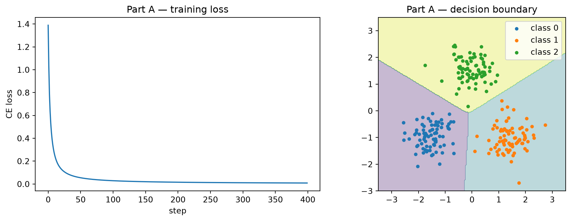
Part A: training-loss curve and decision boundary of the MLP-from-scratch on the 2-D blobs.
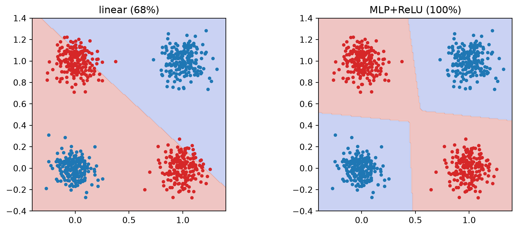
Part B: side-by-side decision boundaries of the linear vs ReLU model on XOR, with final accuracy printed for each.
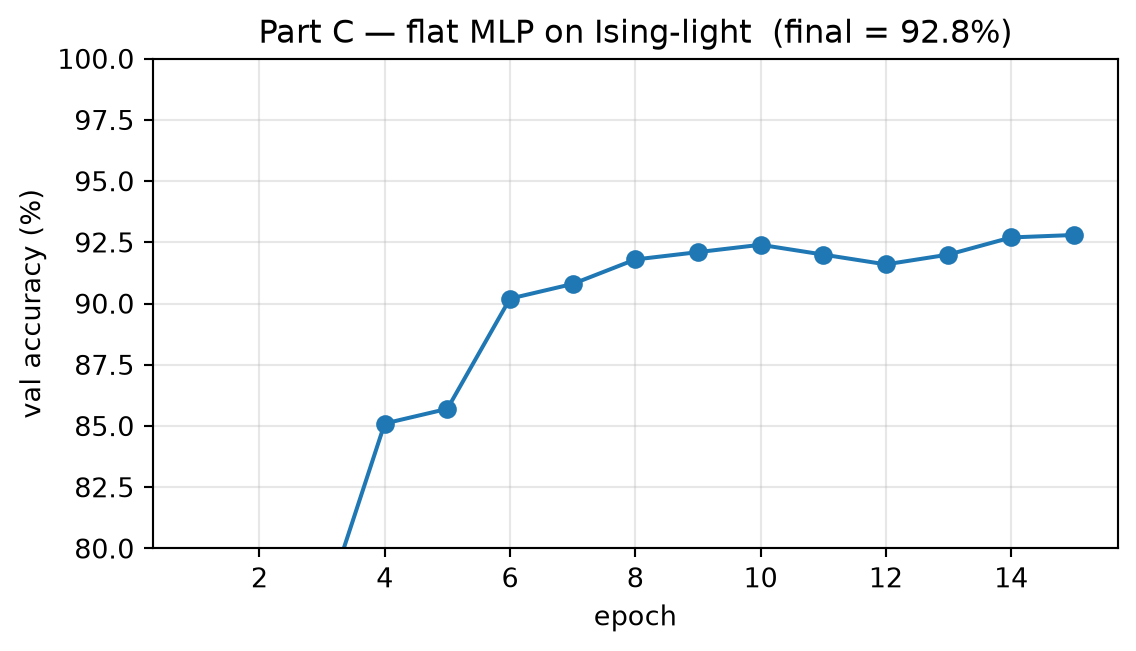
Part C: validation-accuracy curve of the flat MLP on Ising-light, with the final accuracy printed.
Part D: your written answer to the parameter-count question (1 paragraph).
# Standard imports for the whole homework. Same idiom as weeks 2 and 3.import numpy as npimport torchimport torch.nn as nnimport torch.nn.functional as Ffrom torch.utils.data import DataLoader, random_splitimport matplotlib.pyplot as pltfrom ai4mat.datasets import IsingDatasetnp.random.seed(0)torch.manual_seed(0)
<torch._C.Generator at 0x7f94f0765fd0>
Part A — A 2-layer MLP from scratch
We build a tiny multi-layer perceptron withoutnn.Linear or nn.Sequential. The point is to see, in one screen of code, that a “neural network” really is just affine → activation → affine. We then confirm autograd computes the gradients we’d compute by hand.
(see MFML §“A dense layer”)
# Synthesize a small 2-D 3-class blob dataset so we can visualise the boundary.rng = np.random.default_rng(0)n_per_class =80centers = np.array([[-1.5, -1.0], [1.5, -1.0], [0.0, 1.5]])X_np = np.vstack([rng.normal(c, 0.45, (n_per_class, 2)) for c in centers])y_np = np.repeat(np.arange(3), n_per_class)X = torch.tensor(X_np, dtype=torch.float32)y = torch.tensor(y_np, dtype=torch.long)print(f"X shape: {tuple(X.shape)} y shape: {tuple(y.shape)} classes: {y.unique().tolist()}")
X shape: (240, 2) y shape: (240,) classes: [0, 1, 2]
# A 2-layer MLP from scratch. Hidden width H=16, ReLU activation,# 3-class softmax output. Parameters are leaf tensors with requires_grad.torch.manual_seed(0)H =16W1 = (torch.randn(2, H) *0.5).requires_grad_(True)b1 = torch.zeros(H, requires_grad=True)W2 = (torch.randn(H, 3) *0.5).requires_grad_(True)b2 = torch.zeros(3, requires_grad=True)def forward_scratch(x):"""Forward pass implemented in plain torch ops -- no nn.Module.""" z1 = x @ W1 + b1 # (N, H) h = torch.relu(z1) # (N, H) z2 = h @ W2 + b2 # (N, 3)return z2 # logits; softmax happens inside CrossEntropyLoss
# Sanity-check by comparing to an `nn.Sequential` with the *same* weights.ref = nn.Sequential(nn.Linear(2, H), nn.ReLU(), nn.Linear(H, 3))with torch.no_grad(): ref[0].weight.copy_(W1.t()); ref[0].bias.copy_(b1) ref[2].weight.copy_(W2.t()); ref[2].bias.copy_(b2)with torch.no_grad(): delta = (forward_scratch(X) - ref(X)).abs().max().item()print(f"max |scratch - nn.Sequential| = {delta:.2e} (should be 0 up to fp noise)")
max |scratch - nn.Sequential| = 3.58e-07 (should be 0 up to fp noise)
# Train it with vanilla GD on the full batch. Cross-entropy = NLL of softmax,# computed in a numerically stable way by PyTorch's F.cross_entropy.lr =0.1hist_loss = []for step inrange(400): logits = forward_scratch(X) loss = F.cross_entropy(logits, y)# Manual zero-grad + backward + step.for p in (W1, b1, W2, b2):if p.grad isnotNone: p.grad.zero_() loss.backward()with torch.no_grad():for p in (W1, b1, W2, b2): p -= lr * p.grad hist_loss.append(loss.item())acc = (forward_scratch(X).argmax(dim=1) == y).float().mean().item()print(f"final train accuracy: {acc *100:.1f}% final loss: {hist_loss[-1]:.4f}")
final train accuracy: 100.0% final loss: 0.0085
# Plot the loss curve and the decision boundary.xx, yy = np.meshgrid(np.linspace(-3.5, 3.5, 200), np.linspace(-3.0, 3.5, 200))grid = torch.tensor(np.stack([xx.ravel(), yy.ravel()], axis=1), dtype=torch.float32)with torch.no_grad(): pred = forward_scratch(grid).argmax(dim=1).numpy().reshape(xx.shape)fig, axes = plt.subplots(1, 2, figsize=(11, 4))axes[0].plot(hist_loss); axes[0].set_xlabel("step"); axes[0].set_ylabel("CE loss")axes[0].set_title("Part A — training loss")axes[1].contourf(xx, yy, pred, alpha=0.3, cmap="viridis")for k, color inzip(range(3), ["tab:blue", "tab:orange", "tab:green"]): axes[1].scatter(X_np[y_np == k, 0], X_np[y_np == k, 1], s=12, c=color, label=f"class {k}")axes[1].legend(); axes[1].set_aspect("equal"); axes[1].set_title("Part A — decision boundary")plt.tight_layout(); plt.show()
What you should see. Loss drops from ~1.1 to ~0.05 over 400 steps; final accuracy ~99-100%. The decision boundary is non-linear — three regions whose borders are piecewise linear. Each kink corresponds to a hidden ReLU activating. With only 16 hidden units you can already see the geometric vocabulary the network is using to carve up the input space.
(see MFML §“Activation functions: what we need today”)
Part B — XOR drill: why non-linearity is non-negotiable
XOR is the textbook task that proved (Minsky & Papert, 1969) you cannot solve every problem with a single linear layer. We replicate it in two minutes:
The four corners of a square get labels \(\{0, 1, 1, 0\}\) — perfectly separable, but not by a hyperplane.
A single nn.Linear(2, 2) followed by softmax can never achieve > 50% accuracy.
A two-layer MLP with any non-linearity cracks it instantly.
(see MFML §“Why non-linearity is non-negotiable”)
# Build a noisy XOR dataset: 200 points around each corner of a unit square.torch.manual_seed(1)rng = np.random.default_rng(1)corners = np.array([[0.0, 0.0], [1.0, 0.0], [0.0, 1.0], [1.0, 1.0]])labels = np.array([0, 1, 1, 0])n =200Xx_np = np.vstack([rng.normal(c, 0.10, (n, 2)) for c in corners])yx_np = np.repeat(labels, n)Xx = torch.tensor(Xx_np, dtype=torch.float32)yx = torch.tensor(yx_np, dtype=torch.long)
# Train two models: a single linear layer (logistic regression in 2-D) and a# small MLP. Identical optimizer / loss / data — only the architecture differs.def train_model(model, X_, y_, epochs=400, lr=0.1): opt = torch.optim.SGD(model.parameters(), lr=lr) loss_fn = nn.CrossEntropyLoss()for _ inrange(epochs): opt.zero_grad() loss = loss_fn(model(X_), y_) loss.backward() opt.step()with torch.no_grad(): acc = (model(X_).argmax(dim=1) == y_).float().mean().item()return acclin_model = nn.Linear(2, 2)mlp_model = nn.Sequential(nn.Linear(2, 8), nn.ReLU(), nn.Linear(8, 2))acc_lin = train_model(lin_model, Xx, yx)acc_mlp = train_model(mlp_model, Xx, yx)print(f"linear accuracy: {acc_lin *100:5.1f}% <-- ~50%, no better than chance")print(f"MLP+ReLU accuracy: {acc_mlp *100:5.1f}% <-- ~100%, the hidden layer fixes it")
linear  accuracy:  68.3%   <-- ~50%, no better than chance
MLP+ReLU accuracy: 100.0%   <-- ~100%, the hidden layer fixes it
The take-home. A linear model can only draw straight boundaries. XOR requires two such boundaries combined with an OR — which is exactly what one hidden ReLU layer expresses. Non-linearity is not decoration. Without it, every neural network — no matter how deep — collapses back to a single linear map (composition of linear maps is linear).
(see MFML §“Activation functions” and the “warping rings” interactive)
Part C — nn.Sequential idiom + Ising-light flat MLP baseline
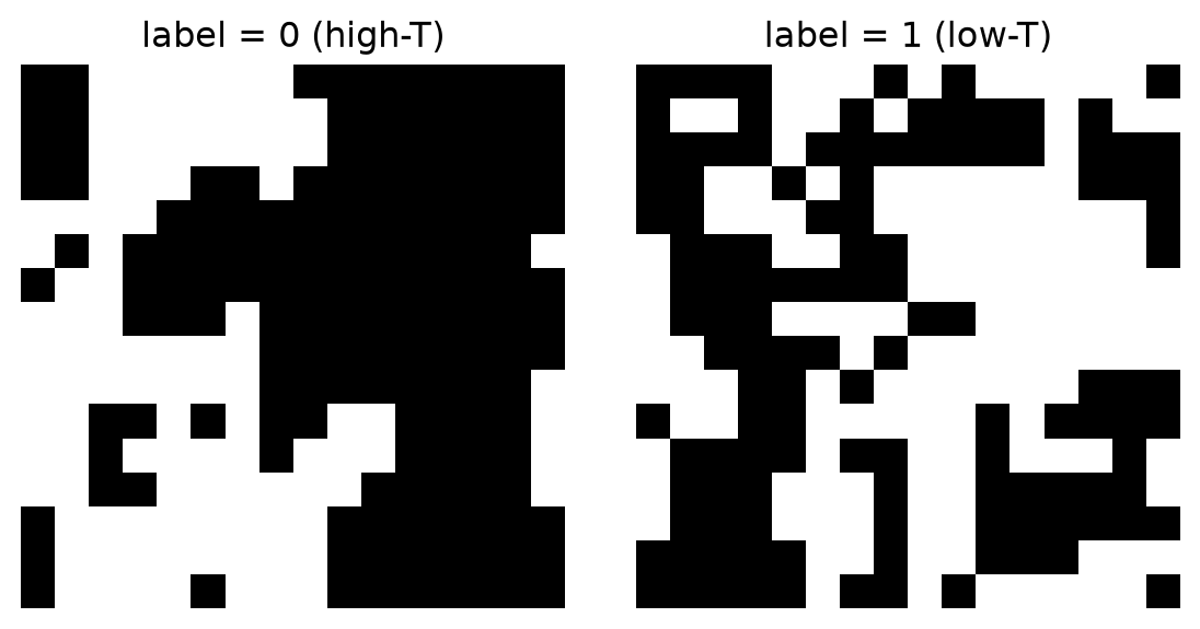
Now we move from synthetic toy data to a real(-ish) materials problem: the Ising microstructure dataset — \(16 \times 16\) binary spin configurations labelled high-temperature (paramagnetic, label 0) vs low-temperature (ferromagnetic, label 1). This is the same dataset we will iterate on Thursday with a CNN.
Today’s question: how well does a plain flat MLP do on raw pixels?
(see MFML §“From historical neuron to modern layer” → §“Dense networks learn features”; ML-PC §“Image as Tensor”)
# Load the dataset. IsingDataset provides X of shape (1, 16, 16) per sample.ds = IsingDataset(size="light")print(f"size: {len(ds)} image shape: {tuple(ds[0][0].shape)} labels: {ds.y.unique().tolist()}")# Train/val split with a fixed generator for reproducibility.gen = torch.Generator().manual_seed(0)n_train =int(0.8*len(ds))n_val =len(ds) - n_traintrain_ds, val_ds = random_split(ds, [n_train, n_val], generator=gen)train_loader = DataLoader(train_ds, batch_size=128, shuffle=True, generator=torch.Generator().manual_seed(0))val_loader = DataLoader(val_ds, batch_size=256, shuffle=False)print(f"train={n_train} val={n_val}")
# Train. Standard supervised loop: Adam, cross-entropy, log val accuracy.def evaluate(model, loader): model.eval() correct = total =0with torch.no_grad():for x, y_ in loader: correct += (model(x).argmax(dim=1) == y_).sum().item() total += y_.numel()return correct / totalopt = torch.optim.Adam(flat_mlp.parameters(), lr=1e-3)loss_fn = nn.CrossEntropyLoss()val_hist = []for epoch inrange(15): flat_mlp.train()for x, y_ in train_loader: opt.zero_grad() loss = loss_fn(flat_mlp(x), y_) loss.backward() opt.step() val_hist.append(evaluate(flat_mlp, val_loader))print(f"epoch {epoch +1:2d} val acc = {val_hist[-1] *100:5.2f}%")
epoch  1   val acc = 75.70%
epoch  2   val acc = 79.30%
epoch  3   val acc = 77.30%
epoch  4   val acc = 85.10%
epoch  5   val acc = 85.70%
epoch  6   val acc = 90.20%
epoch  7   val acc = 90.80%
epoch  8   val acc = 91.80%
epoch  9   val acc = 92.10%
epoch 10   val acc = 92.40%
epoch 11   val acc = 92.00%
epoch 12   val acc = 91.60%
epoch 13   val acc = 92.00%
epoch 14   val acc = 92.70%
epoch 15   val acc = 92.80%
fig, ax = plt.subplots(figsize=(6, 3.5))ax.plot(range(1, len(val_hist) +1), [v *100for v in val_hist], "o-")ax.set_xlabel("epoch"); ax.set_ylabel("val accuracy (%)")ax.set_title(f"Part C — flat MLP on Ising-light (final = {val_hist[-1] *100:.1f}%)")ax.set_ylim(80, 100); ax.grid(True, alpha=0.3)plt.tight_layout(); plt.show()
What you should see. The flat MLP gets to roughly 90–95% val accuracy in 15 epochs. Decent — but on Thursday we will see that the same dataset can be solved with fewer parameters by a CNN, and with one number by a linear classifier on hand-crafted mean magnetization. The gap between those three numbers is the entire content of MLPC Unit 4.
Part D — The dense-image problem (parameter-count reflection)
Imagine we want to train an MLP on the full Ising dataset, where images are \(64 \times 64\) instead of \(16 \times 16\). Compute the parameter count of a single fully-connected layer that maps the flattened image to a 256-unit hidden vector — and compare it to the parameters of a 3-layer CNN that we will build on Thursday (channels 8 → 16 → 32, all with \(3 \times 3\) kernels).
(see MFML §“The dense image problem” and §“Parameter economy”)
# Numbers below are the answer template -- fill in your computation in Markdown.def mlp_first_layer_params(input_pixels: int, hidden: int) ->int:"""An nn.Linear has weight (out, in) + bias (out,)."""return hidden * input_pixels + hiddendef conv_block_params(in_ch: int, out_ch: int, k: int) ->int:"""Conv2d(in_ch, out_ch, k) has weight (out, in, k, k) + bias (out,)."""return out_ch * in_ch * k * k + out_chprint("=== MLP first layer (flatten -> 256 hidden) ===")print(f" 16x16 image: {mlp_first_layer_params(16*16, 256):>10,} params")print(f" 64x64 image: {mlp_first_layer_params(64*64, 256):>10,} params")print(f" 256x256 image: {mlp_first_layer_params(256*256, 256):>10,} params")print()print("=== Tiny 3-layer CNN (channels 1 -> 8 -> 16 -> 32, 3x3 kernels) ===")cnn_params = ( conv_block_params(1, 8, 3)+ conv_block_params(8, 16, 3)+ conv_block_params(16, 32, 3))print(f" CNN feature extractor: {cnn_params:,} params (independent of image size!)")
Answer the following in your own words. Bring your written answer to class on Thursday.
By how many orders of magnitude does the MLP first-layer parameter count grow when the image goes from \(16 \times 16\) to \(256 \times 256\)?
What does the CNN parameter count do as the image grows? Why?
In one sentence: which assumption about the data is the CNN exploiting that the MLP is not?
Hint: the answer to (3) is two words and is the title of MFML §“Weight sharing gives convolution”.
Done — see you Thursday
On Thursday we’ll cash in this homework:
Block 1 reuses your Part C result as the flat-MLP baseline.
Block 2 verifies your Part D parameter explosion with measured run-time.
Block 3 hand-builds a convolution layer with F.conv2d.
Blocks 4–6 turn it into a tiny CNN and compare three different representations of the same Ising labels — culminating in the one-number scalar that beats every neural network we’ll have built.