MFML Unit 5: Clustering and autoencoders — K-means and Lloyd’s algorithm, the GMM/EM relaxation, PCA as a linear autoencoder, the non-linear autoencoder bottleneck.
ML-PC Unit 5: Unsupervised learning in materials — applying these methods to unlabelled lab data, validating without ground truth, and using reconstruction error as an anomaly score for distribution shift.
Red thread:K-means quantises data into K discrete codes; an autoencoder quantises into a continuous code. Both ask the same question — “what is the smallest description of \(\mathbf{x}\) that still lets us recognise it?” — answered with hard labels (K-means), soft probabilities (GMM/EM), and learned latent vectors (autoencoder). Today we run all three on the same Ising microstructure data and compare what each one discovers without ever seeing a phase label.
Pre-flight check. This notebook assumes you have run notebooks/week5_homework.py. Block 1 picks up directly from your Lloyd loop and Part C nanoindentation result; we will not re-derive them.
Agenda (90 min)
Block
Min
Topic
1
~6
Recap from homework — Lloyd on blobs, K-means on nanoindentation (low ARI), and today’s three moves
2
~12
Hard → soft assignments: GMM/EM, responsibilities, BIC for K
3
~10
K-means as the σ²→0 limit of an isotropic GMM
4
~8
PCA on NEU-DET — the linear baseline (and why it is not enough)
5
~14
A tiny convolutional autoencoder on NEU-DET; latent scatter; honest read
5b
~8
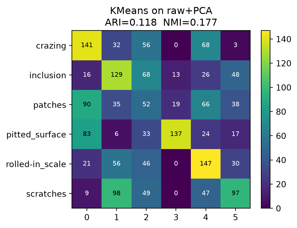
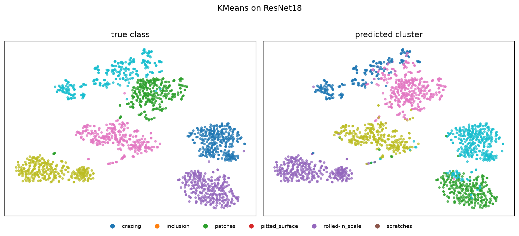
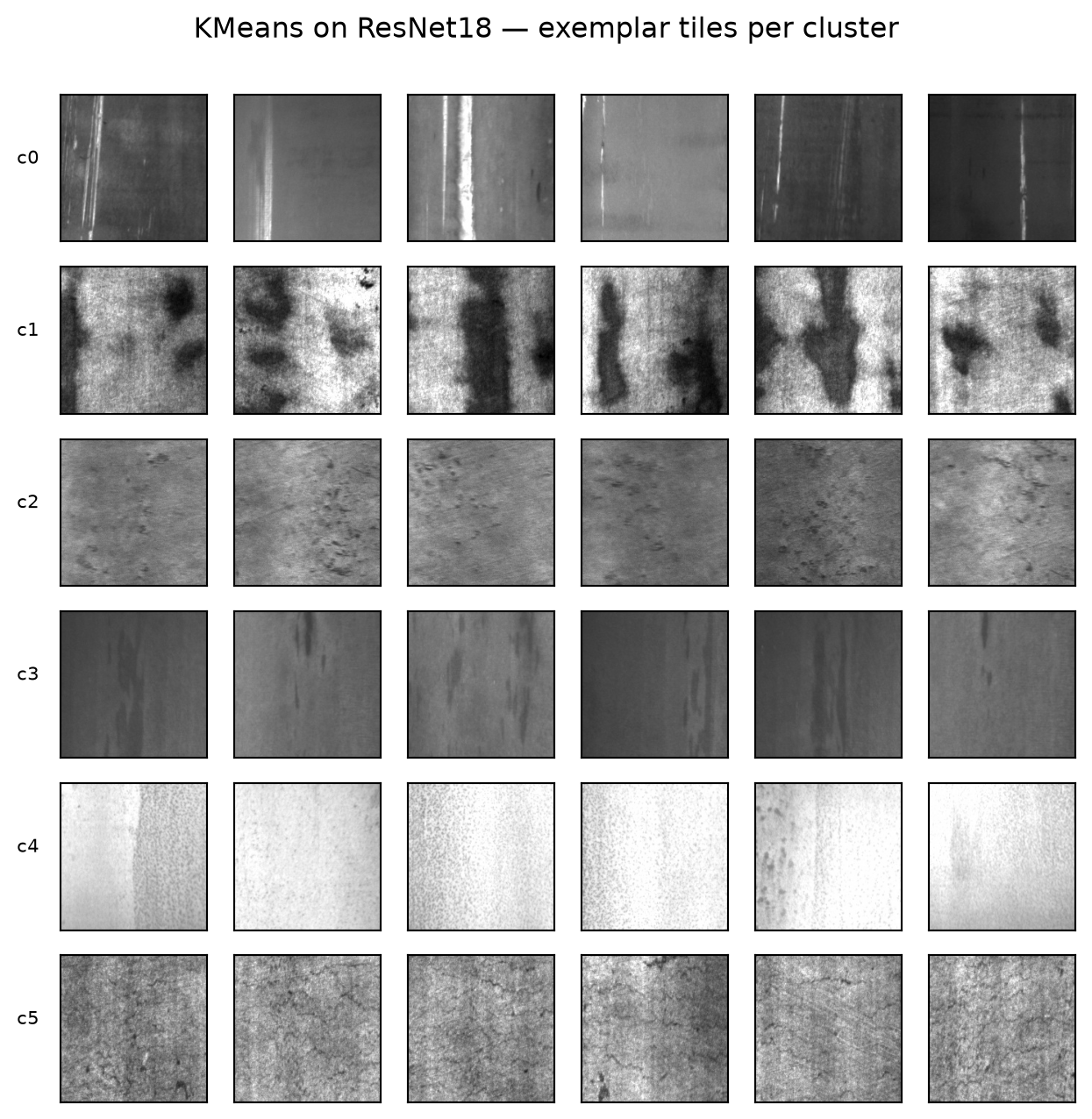
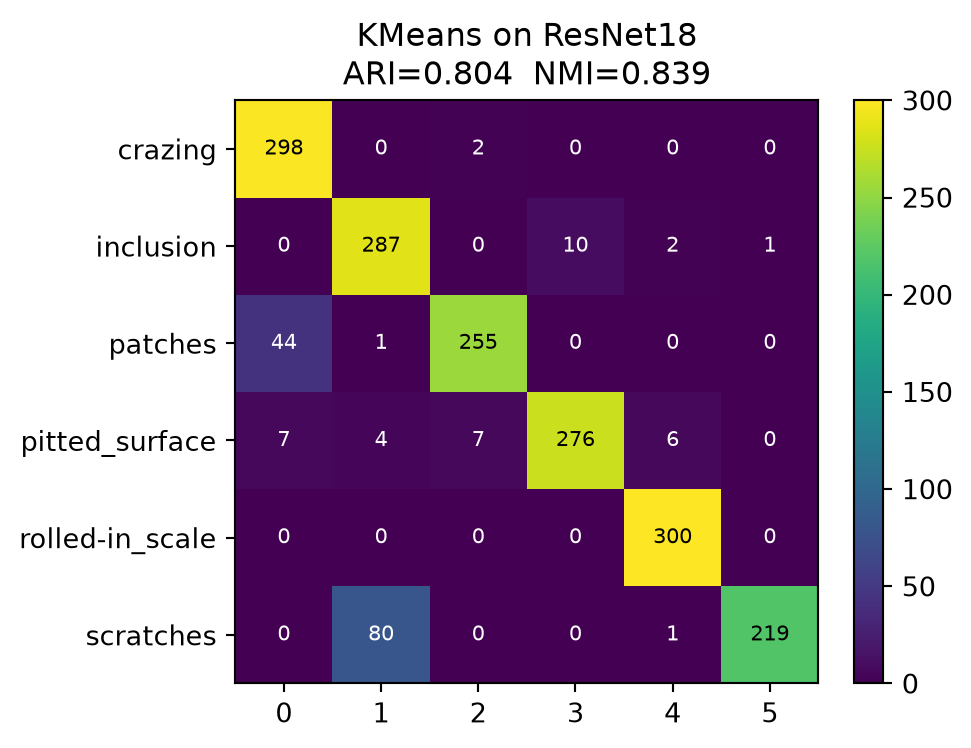
K-means / GMM on NEU-DET features: raw+PCA vs frozen ResNet18 (representation beats algorithm)
6
~8
Reconstruction error as anomaly score — NEU-DET vs Cahn–Hilliard
7
~24
Student exercises (3 core + 1 stretch)
# Standard imports. Same idiom as weeks 2-4: explicit seeds, no hidden state.import numpy as npimport torchimport torch.nn as nnimport torch.nn.functional as Ffrom torch.utils.data import DataLoader, TensorDataset, random_splitimport matplotlib.pyplot as pltfrom sklearn.datasets import make_blobsfrom sklearn.cluster import KMeansfrom sklearn.mixture import GaussianMixturefrom sklearn.metrics import adjusted_rand_score, roc_auc_score, roc_curvefrom ai4mat.datasets import NEUDETDataset, NanoindentationDataset, CahnHilliardDatasetnp.random.seed(0)torch.manual_seed(0)USE_CUDA =TrueDEVICE = torch.device("cuda"if USE_CUDA and torch.cuda.is_available() else"cpu")print(f"Using device: {DEVICE}")
Using device: cpu
Helpers used by every block
def standardise(z, dim=0):"""Return (z - mean) / std along `dim`. Used for clustering preprocessing.""" mu = z.mean(dim=dim, keepdim=True) sd = z.std(dim=dim, keepdim=True)return (z - mu) / (sd +1e-12)def n_params(model) ->int:returnsum(p.numel() for p in model.parameters() if p.requires_grad)
Block 1 — Recap from homework, and today’s question
In Part A you implemented Lloyd’s algorithm in two NumPy lines and watched the centroids migrate on 2-D blobs. In Part C you ran the same algorithm twice on the same real materials data — K-means K=4 on NanoindentationDataset, raw vs standardised — and discovered something uncomfortable: synthetic blobs (C.1) showed standardisation matters a lot when feature scales differ, but on the real Cu/Cr nanoindentation (C.2) standardisation barely moved ARI: both runs landed around 0.1. The Cr-content labels do not live in \((E, H)\) geometry, and no rescaling can conjure them.
We restate the C.2 result in 6 lines so the rest of the lecture has a baseline to push against.
Today’s question. When K-means on the features we have cannot recover the labels we want, what are the moves available to us?
Relax the assignment → GMM/EM (Block 2), and the realisation that K-means is just GMM with isotropic \(\sigma^2\!\to\!0\) covariances (Block 3).
Change the representation → leave 2-D feature tables behind and work on image data (NEU-DET steel-surface defects), comparing PCA (Block 4), a from-scratch conv-AE (Block 5), and pretrained ResNet18 features (Block 5b).
Change the question → use the AE’s reconstruction error as an OOD anomaly score rather than chasing semantic labels (Block 6).
(see MFML §“Lloyd’s algorithm”; ML-PC §“What unsupervised buys you”, §“Validation problem without labels”)
ds_nano = NanoindentationDataset()Xn = ds_nano.X.numpy()yn = ds_nano.y.numpy()Xn_std = (Xn - Xn.mean(axis=0)) / Xn.std(axis=0)km4 = KMeans(n_clusters=4, n_init=10, random_state=0).fit(Xn_std)ari_km = adjusted_rand_score(yn, km4.labels_)print(f"recap (homework C.2): K-means K=4 on standardised (E, H) ARI = {ari_km:.3f}")print(" (low — labels are not in the (E, H) geometry; this is the baseline today's blocks push against)")
recap (homework C.2): K-means K=4 on standardised (E, H)   ARI = 0.111
                       (low — labels are not in the (E, H) geometry; this is the baseline today's blocks push against)
Block 2 — Hard → soft assignments: GMM and EM
K-means hands every point exactly one label. A point sitting between two clusters is forced to commit even when both choices are nearly equally good. A Gaussian mixture model relaxes that commitment: every point gets a probability vector \(\boldsymbol\gamma_i = (\gamma_{i1}, \dots,
\gamma_{iK})\) with \(\sum_k \gamma_{ik} = 1\). The EM algorithm fits the mixture by alternating an E-step (compute the \(\gamma_{ik}\)) and an M-step (re-estimate \(\pi_k, \boldsymbol\mu_k, \boldsymbol\Sigma_k\)).
We use sklearn.mixture.GaussianMixture here — the algorithm is exactly the EM you saw in MFML §E “EM — E-step and M-step”. We focus on the two things that are new compared to K-means: (i) soft membership, and (ii) the BIC as a principled, likelihood-based way to choose K.
(see MFML §“The Gaussian Mixture Model”, §“EM — E-step and M-step”)
# Two overlapping, anisotropic 2-D clusters — the kind of data K-means# struggles with and a full-covariance GMM handles cleanly.rng = np.random.default_rng(7)A = rng.multivariate_normal([-1.0, 0.0], [[0.6, 0.3], [0.3, 0.4]], 200)B = rng.multivariate_normal([+1.5, 0.5], [[0.5, -0.2], [-0.2, 0.8]], 200)X_overlap = np.vstack([A, B])y_overlap = np.array([0] *200+ [1] *200)gmm = GaussianMixture(n_components=2, covariance_type="full", random_state=0).fit(X_overlap)gamma = gmm.predict_proba(X_overlap) # (N, 2) responsibilitiesprint(f"GMM converged in {gmm.n_iter_} EM iterations log-lik = {gmm.score(X_overlap)*len(X_overlap):.1f}")print(f"mixing weights pi = {gmm.weights_.round(3)}")
GMM converged in 4 EM iterations   log-lik = -1019.0
mixing weights pi = [0.524 0.476]
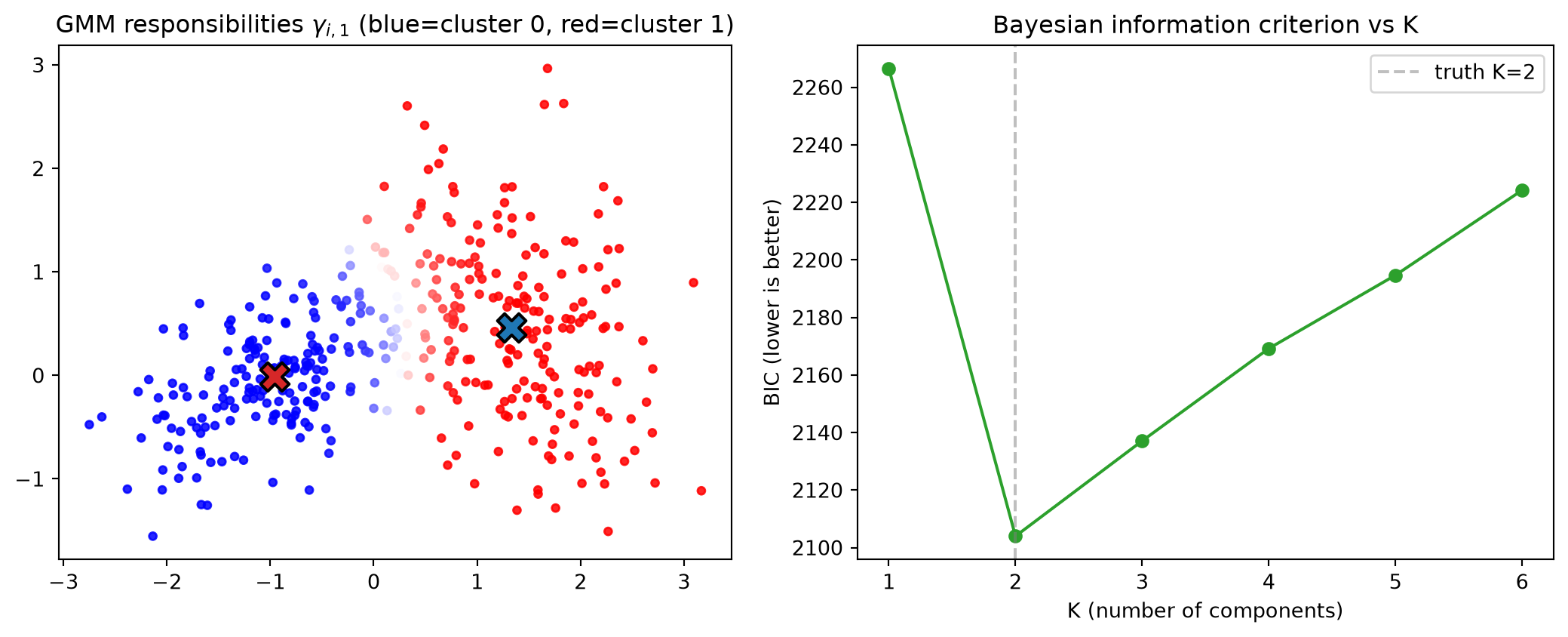
# Plot soft-assignment heatmap on the overlap region.fig, axes = plt.subplots(1, 2, figsize=(11, 4.5))axes[0].scatter(X_overlap[:, 0], X_overlap[:, 1], c=gamma[:, 0], cmap="bwr", s=14, alpha=0.85, vmin=0, vmax=1)for k, color inzip(range(2), ["#1f77b4", "#d62728"]): axes[0].scatter(*gmm.means_[k], c=color, s=200, marker="X", edgecolors="k", linewidths=1.5)axes[0].set_title("GMM responsibilities $\\gamma_{i,1}$ (blue=cluster 0, red=cluster 1)")axes[0].set_aspect("equal")# BIC vs K on the same data — the model-selection diagnostic.K_range =list(range(1, 7))bics = []for K in K_range: g = GaussianMixture(n_components=K, covariance_type="full", random_state=0).fit(X_overlap) bics.append(g.bic(X_overlap))axes[1].plot(K_range, bics, "o-", color="#2ca02c")axes[1].set_xlabel("K (number of components)"); axes[1].set_ylabel("BIC (lower is better)")axes[1].axvline(2, color="gray", ls="--", alpha=0.5, label="truth K=2")axes[1].legend(); axes[1].set_title("Bayesian information criterion vs K")plt.tight_layout()plt.show()
Read the responsibility heatmap. Points deep in either cluster get \(\gamma \approx 0\) or \(\gamma \approx 1\); points in the overlap zone get \(\gamma \approx 0.5\). The model honestly says “I’m not sure” exactly where we would expect — that uncertainty is the upgrade soft assignments buy over hard ones, and it is exactly the property exam Q5 tests in MFML.
Block 3 — K-means as a special case of GMM
MFML §“K-Means is a special case of GMM” claimed that K-means is what you get from a GMM if you (i) fix every covariance to \(\boldsymbol\Sigma_k =
\sigma^2 \mathbf{I}\) (isotropic, equal width across clusters), and (ii) let \(\sigma^2 \to 0\). We verify the claim numerically: a tiny-\(\sigma\)spherical-covariance GMM and a K-means run on the same data should produce the same hard assignment.
(see MFML §“K-Means is a special case of GMM”)
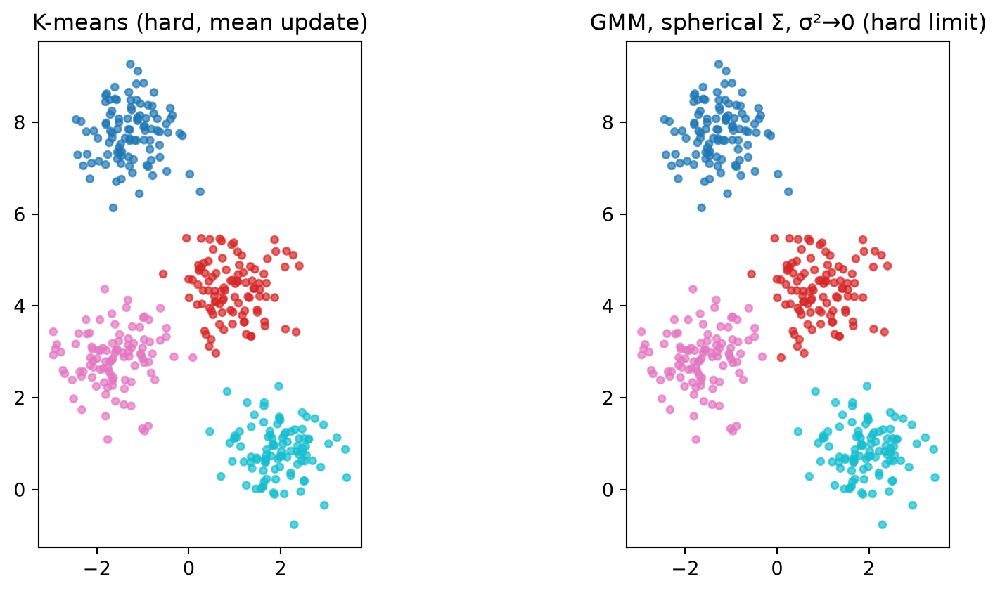
X_blob, _ = make_blobs(n_samples=400, centers=4, cluster_std=0.6, random_state=0)km_blob = KMeans(n_clusters=4, n_init=10, random_state=0).fit(X_blob)# `spherical` => one scalar variance per component; small `reg_covar` keeps# the variance pinned near zero so we are effectively in the σ²→0 regime.gmm_tight = GaussianMixture( n_components=4, covariance_type="spherical", reg_covar=1e-6, random_state=0).fit(X_blob)# Compare hard assignments (label IDs may permute, so use ARI).labels_km = km_blob.labels_labels_gmm = gmm_tight.predict(X_blob)print(f"agreement (ARI) between K-means and tight-σ spherical GMM: {adjusted_rand_score(labels_km, labels_gmm):.3f}")fig, axes = plt.subplots(1, 2, figsize=(10, 4.5))for ax, lbl, title inzip(axes, [labels_km, labels_gmm], ["K-means (hard, mean update)","GMM, spherical Σ, σ²→0 (hard limit)"]): ax.scatter(X_blob[:, 0], X_blob[:, 1], c=lbl, cmap="tab10", s=14, alpha=0.7) ax.set_title(title); ax.set_aspect("equal")plt.tight_layout()plt.show()
agreement (ARI) between K-means and tight-σ spherical GMM: 0.993
Take-away. ARI ≈ 1: the two assignments coincide up to a permutation of cluster labels. K-means is not “a different algorithm from GMM” — it is GMM with maximally constrained covariances and zero soft-assignment temperature. This is the first clean example in the course of “simple algorithm = limit of richer probabilistic model”; the same pattern returns in MFML Unit 7 (probabilistic view of learning) and Unit 11 (unsupervised learning, contrastive losses).
Block 4 — PCA on NEU-DET — the linear baseline
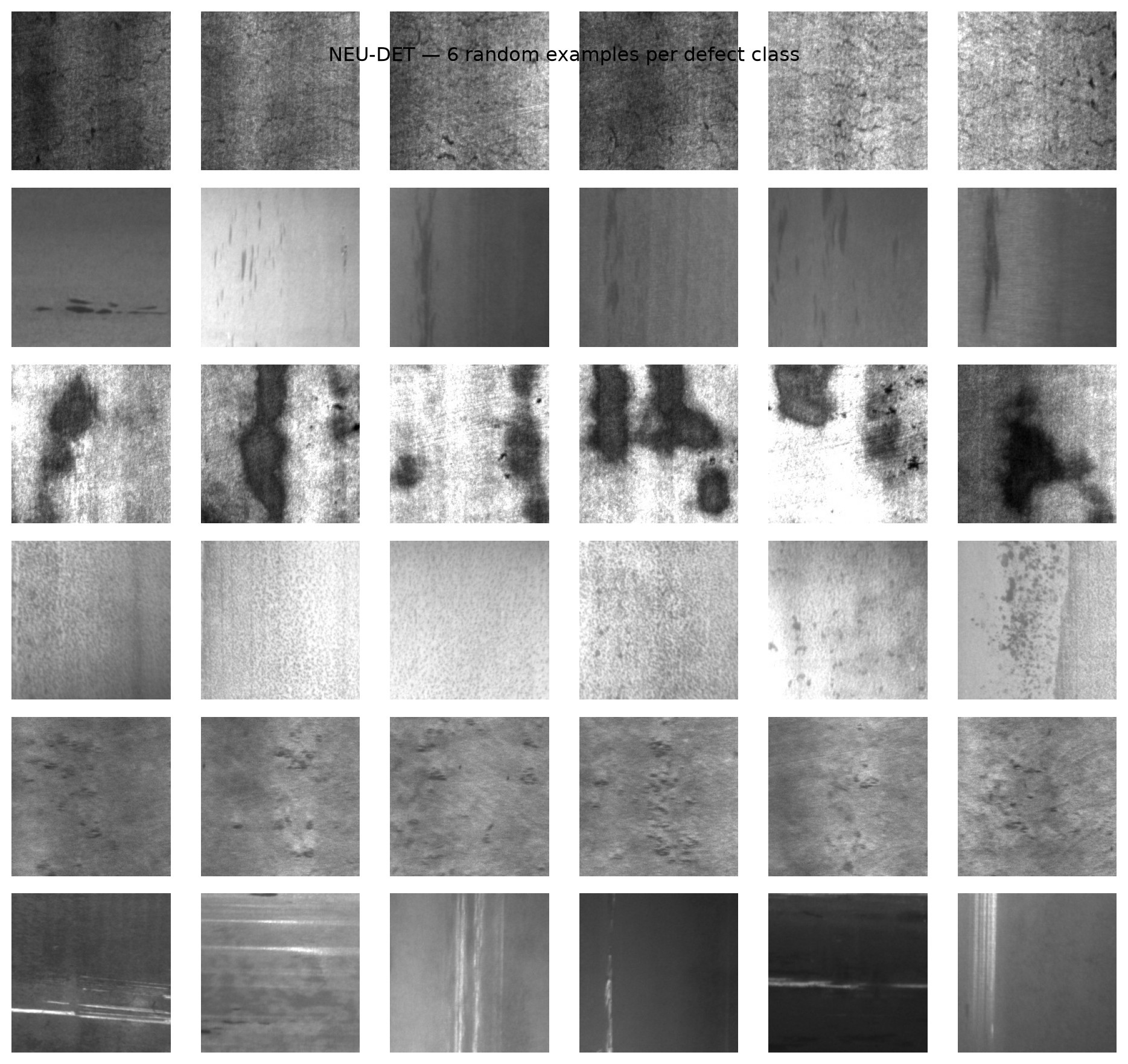
Now we leave 2-D feature tables behind and do unsupervised learning on real microstructure images. NEUDETDataset gives 1,800 grayscale 200×200 steel-surface patches across six defect classes (crazing, inclusion, patches, pitted-surface, rolled-in-scale, scratches). We will pretend we do not know the labels.
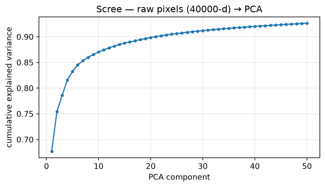
The classical first move is PCA: flatten each 200×200 image into a 40,000-D vector, take the top-2 principal components, and look at the scatter. PCA is the linear autoencoder (encoder = \(\mathbf{U}_k^\top\), decoder = \(\mathbf{U}_k\), MSE) — it is the right baseline to argue against before reaching for a neural network.
(see MFML §“Recap — PCA from Unit 2”, §“Why PCA fails on a manifold”)
ds_neu = NEUDETDataset(root="Ai4MatLectures/data/NEU-DET", split="all", download=True)AE_IMAGE_SIZE = (200, 200)X_img = ds_neu.Xy_img = ds_neu.yprint(f"NEU-DET: N={len(ds_neu)} image shape={tuple(ds_neu.X[0].shape)} "f"classes={ds_neu.class_names}")# Flatten to (N, 40000) and run PCA via torch.pca_lowrank (no sklearn, no# n^2 covariance matrix in memory).Xf = X_img.reshape(len(X_img), -1) # (N, 40000)Xf = Xf - Xf.mean(dim=0, keepdim=True) # centreU, S, V = torch.pca_lowrank(Xf, q=8, center=False)Z_pca = Xf @ V[:, :2] # (N, 2)print(f"top-2 singular values (proxy for explained variance): {S[:2].tolist()}")
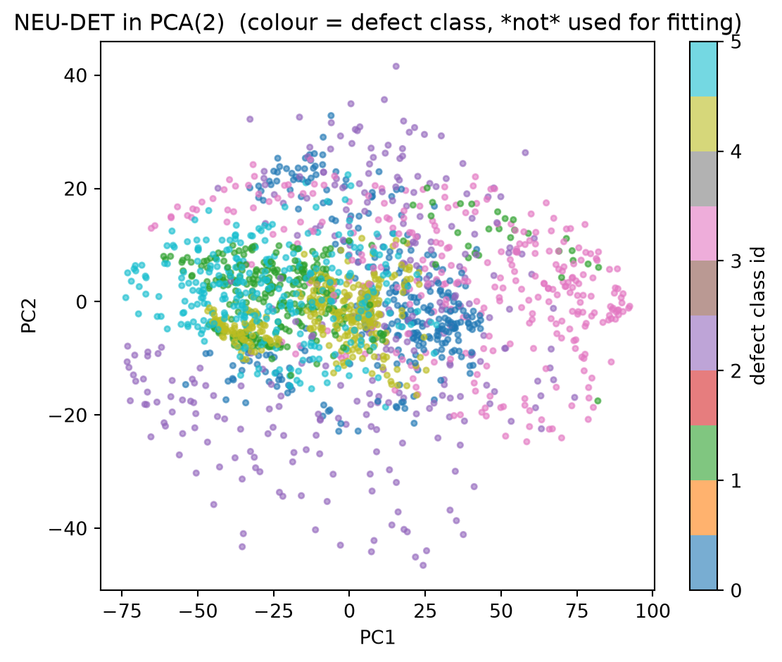
fig, ax = plt.subplots(figsize=(6, 5))sc = ax.scatter(Z_pca[:, 0], Z_pca[:, 1], c=y_img.numpy(), cmap="tab10", s=8, alpha=0.6)ax.set_xlabel("PC1"); ax.set_ylabel("PC2")ax.set_title("NEU-DET in PCA(2) (colour = defect class, *not* used for fitting)")plt.colorbar(sc, ax=ax, label="defect class id")plt.tight_layout()plt.show()
Read this plot. PCA picks the 2-D plane of maximum variance. On NEU-DET that plane separates patches by overall brightness/contrast (PC1 ≈ mean patch intensity, PC2 ≈ low-frequency layout) — but the six defect classes overlap heavily and most of the visually distinctive information (crack networks, pit clusters, scratch orientation) lives in higher-frequency texture, which a linear projection of raw pixels is structurally unable to capture. That is the gap a non-linear autoencoder is built to close (Block 5), and where pretrained image features really earn their keep (Block 5b).
Block 5 — A tiny convolutional autoencoder on NEU-DET
Replace PCA’s linear \(\mathbf{U}_k^\top\) by a 3-layer convolutional encoder, and PCA’s linear \(\mathbf{U}_k\) by a 3-layer transposed-convolution decoder. Bottleneck \(k=2\) so we can plot the latent space; train on raw 200×200 defect patches without ever showing the class labels; minimise MSE reconstruction loss.
(see MFML §“The autoencoder concept”, §“Forward pass through an autoencoder”; ML-PC §“From classical to learned representations”)
# Train/val split, loaders. We hold back 1000 images for held-out# reconstruction-error scoring in Block 6.torch.manual_seed(0)gen = torch.Generator().manual_seed(0)ds_img = TensorDataset(X_img, y_img)train_n =int(0.8*len(ds_img))val_n =len(ds_img) - train_ntrain_ds, val_ds = random_split(ds_img, [train_n, val_n], generator=gen)train_loader = DataLoader(train_ds, batch_size=32, shuffle=True, generator=torch.Generator().manual_seed(0))val_loader = DataLoader(val_ds, batch_size=64, shuffle=False)
torch.manual_seed(0)model = ConvAE(k=2).to(DEVICE)print(f"ConvAE params: {n_params(model):,}")opt = torch.optim.Adam(model.parameters(), lr=1e-4)loss_fn = nn.MSELoss()# 70 epochs on GPU (~few minutes) gets a usable latent + readable# reconstructions on NEU-DET; drop to 20–30 if running on CPU.n_epochs =70for epoch inrange(n_epochs): model.train()for x, _ in train_loader: x = x.to(DEVICE) opt.zero_grad() x_hat = model(x) loss = loss_fn(x_hat, x) loss.backward() opt.step() model.eval()with torch.no_grad(): val_loss =0.0for x, _ in val_loader: x = x.to(DEVICE) val_loss += loss_fn(model(x), x).item() * x.size(0) val_loss /=len(val_ds)print(f"epoch {epoch +1} val MSE = {val_loss:.4f}")
ConvAE params: 246,851
epoch 1   val MSE = 0.0391
epoch 2   val MSE = 0.0359
epoch 3   val MSE = 0.0320
epoch 4   val MSE = 0.0282
epoch 5   val MSE = 0.0259
epoch 6   val MSE = 0.0225
epoch 7   val MSE = 0.0212
epoch 8   val MSE = 0.0189
epoch 9   val MSE = 0.0182
epoch 10   val MSE = 0.0170
epoch 11   val MSE = 0.0163
epoch 12   val MSE = 0.0158
epoch 13   val MSE = 0.0154
epoch 14   val MSE = 0.0147
epoch 15   val MSE = 0.0148
epoch 16   val MSE = 0.0143
epoch 17   val MSE = 0.0136
epoch 18   val MSE = 0.0134
epoch 19   val MSE = 0.0131
epoch 20   val MSE = 0.0128
epoch 21   val MSE = 0.0129
epoch 22   val MSE = 0.0131
epoch 23   val MSE = 0.0124
epoch 24   val MSE = 0.0120
epoch 25   val MSE = 0.0120
epoch 26   val MSE = 0.0122
epoch 27   val MSE = 0.0120
epoch 28   val MSE = 0.0118
epoch 29   val MSE = 0.0118
epoch 30   val MSE = 0.0119
epoch 31   val MSE = 0.0118
epoch 32   val MSE = 0.0114
epoch 33   val MSE = 0.0115
epoch 34   val MSE = 0.0114
epoch 35   val MSE = 0.0112
epoch 36   val MSE = 0.0112
epoch 37   val MSE = 0.0111
epoch 38   val MSE = 0.0113
epoch 39   val MSE = 0.0114
epoch 40   val MSE = 0.0112
epoch 41   val MSE = 0.0112
epoch 42   val MSE = 0.0111
epoch 43   val MSE = 0.0114
epoch 44   val MSE = 0.0114
epoch 45   val MSE = 0.0115
epoch 46   val MSE = 0.0111
epoch 47   val MSE = 0.0109
epoch 48   val MSE = 0.0113
epoch 49   val MSE = 0.0110
epoch 50   val MSE = 0.0108
epoch 51   val MSE = 0.0108
epoch 52   val MSE = 0.0110
epoch 53   val MSE = 0.0108
epoch 54   val MSE = 0.0108
epoch 55   val MSE = 0.0109
epoch 56   val MSE = 0.0108
epoch 57   val MSE = 0.0108
epoch 58   val MSE = 0.0110
epoch 59   val MSE = 0.0111
epoch 60   val MSE = 0.0108
epoch 61   val MSE = 0.0110
epoch 62   val MSE = 0.0108
epoch 63   val MSE = 0.0107
epoch 64   val MSE = 0.0107
epoch 65   val MSE = 0.0112
epoch 66   val MSE = 0.0111
epoch 67   val MSE = 0.0108
epoch 68   val MSE = 0.0107
epoch 69   val MSE = 0.0108
epoch 70   val MSE = 0.0108
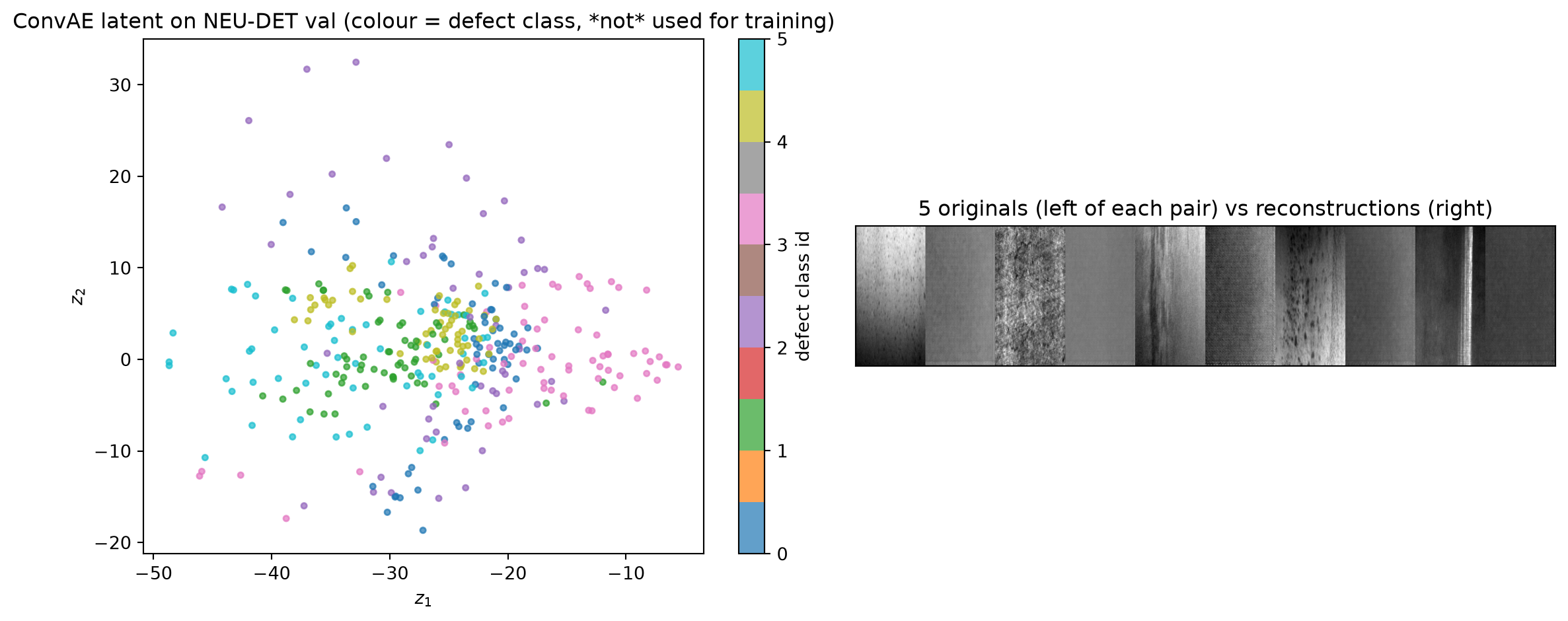
# Encode the held-out validation set into the 2-D latent space and plot,# coloured by the never-seen phase label.model.eval()Z_list, y_list = [], []with torch.no_grad():for x, y in val_loader: x = x.to(DEVICE) Z_list.append(model.encode(x).cpu()) y_list.append(y)Z_ae = torch.cat(Z_list).numpy()Y_ae = torch.cat(y_list).numpy()fig, axes = plt.subplots(1, 2, figsize=(12, 5))sc1 = axes[0].scatter(Z_ae[:, 0], Z_ae[:, 1], c=Y_ae, cmap="tab10", s=10, alpha=0.7)axes[0].set_xlabel("$z_1$"); axes[0].set_ylabel("$z_2$")axes[0].set_title("ConvAE latent on NEU-DET val (colour = defect class, *not* used for training)")plt.colorbar(sc1, ax=axes[0], label="defect class id")# Side-by-side: a few reconstructions to confirm the AE learned defect textures.with torch.no_grad(): x_some, _ =next(iter(val_loader)) x_some = x_some.to(DEVICE) x_hat = model(x_some[:5]).cpu() x_some = x_some.cpu()for i inrange(5): axes[1].imshow(np.hstack([x_some[i, 0].numpy(), x_hat[i, 0].numpy()]), cmap="gray", extent=(i, i +1, 0, 1))axes[1].set_xlim(0, 5); axes[1].set_ylim(0, 1)axes[1].set_xticks([]); axes[1].set_yticks([])axes[1].set_title("5 originals (left of each pair) vs reconstructions (right)")plt.tight_layout()plt.show()
Honest read of this latent space. Training converges — the reconstruction MSE keeps dropping and the right-hand panel shows the decoder does produce defect-like textures. But the 2-D latent does not cleanly separate the six NEU-DET defect classes: most classes overlap in one diffuse blob and only one or two classes drift to the edges.
This is the typical outcome when you train a tiny convolutional autoencoder on a small dataset (1,800 images, 6 classes) from scratch:
The objective is wrong for clustering. MSE on raw pixels rewards reproducing brightness and large-scale layout, not the high-frequency texture cues (cracks, pits, scratches) that actually distinguish classes. The AE happily encodes overall image intensity into the 2-D code and discards what we care about.
The bottleneck is too tight. 2 latent dimensions cannot hold six visually distinct defect modes at once. Increasing \(k\) helps, but the MSE bias above limits how much.
There is no class-discriminative signal in training. The AE is never told that “patches” and “scratches” should land in different regions of latent space; any separation we see is a byproduct of reconstruction, not the goal.
The dataset is small. ~1,500 train images is far below what a convolutional model needs to learn texture-discriminative features from scratch. Pretrained features (Block 5b) sidestep this entirely.
Take-away: a small AE trained from scratch on a small materials dataset can converge without giving us a useful representation for downstream clustering. Block 5b makes this concrete by replacing the AE latent with (i) raw pixels + PCA and (ii) frozen ResNet18 features and re-running the same K-means / GMM evaluation.
Block 5b — Clustering NEU-DET: raw pixels vs ResNet18 embeddings
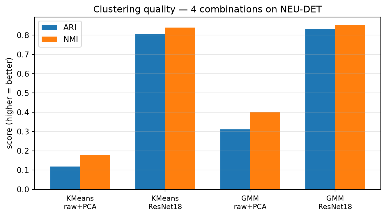
The ConvAE struggles on NEU-DET; this block makes the representation matter explicit. We compare two feature pipelines on the full NEU-DET set:
Raw pixels + PCA(50) — a flat 40,000-D vector, reduced for tractability.
Pretrained ResNet18 embeddings (512-D) — ImageNet features, no fine-tuning.
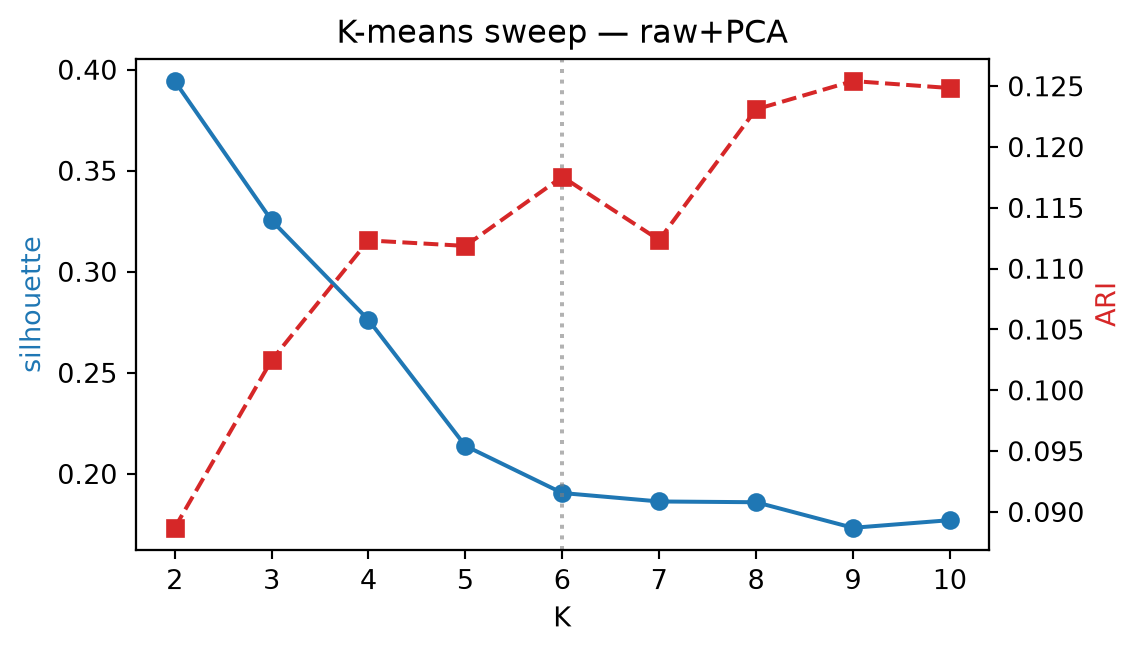
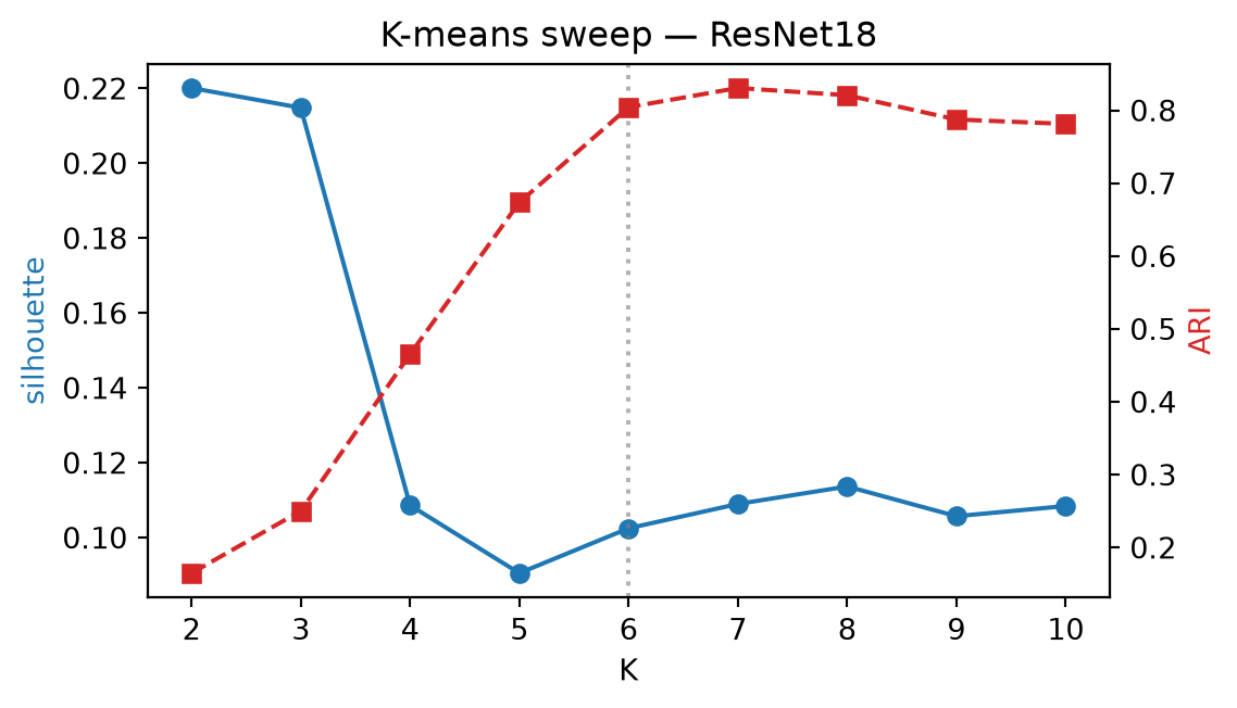
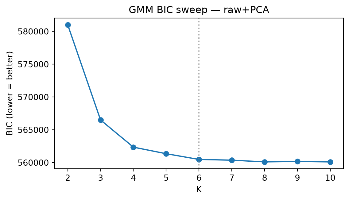
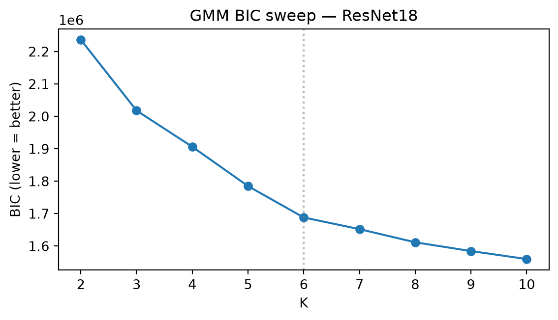
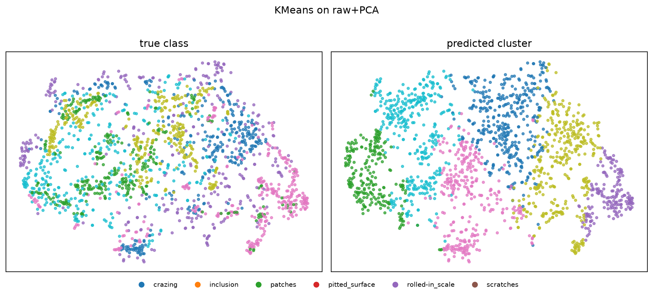
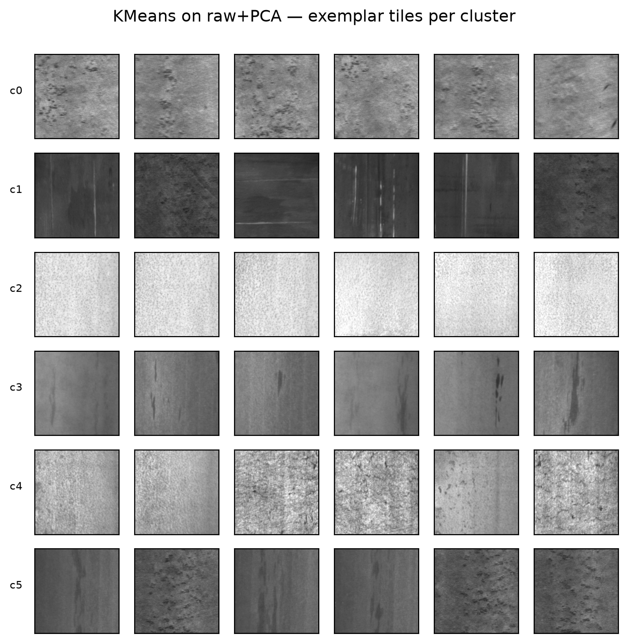
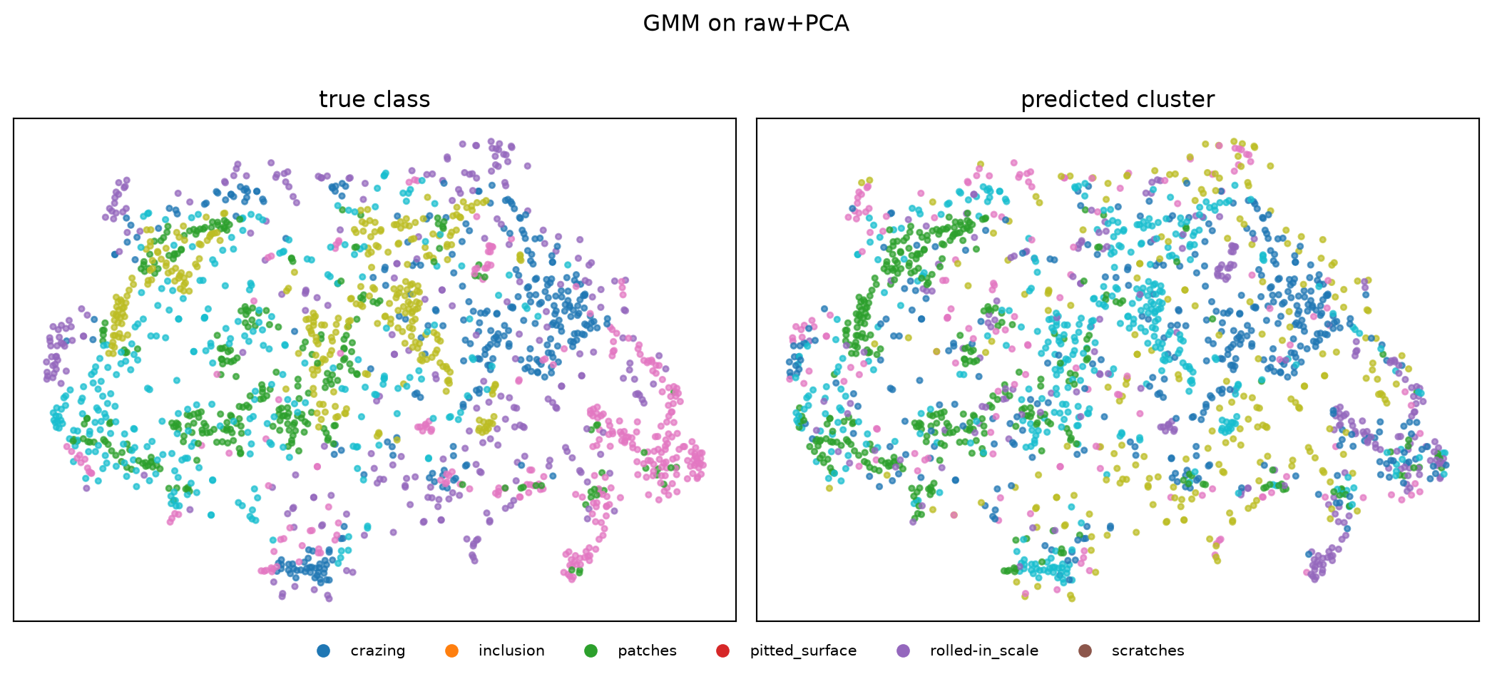
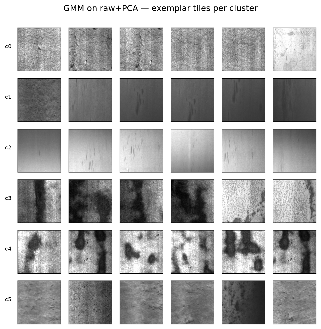
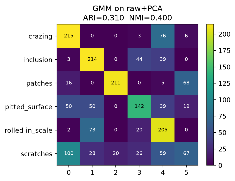
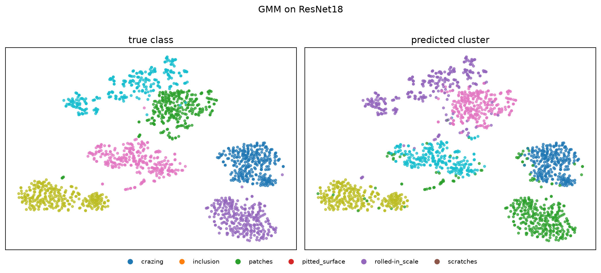
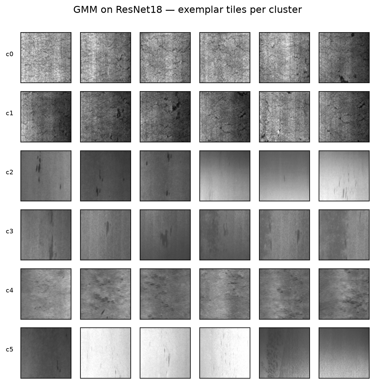
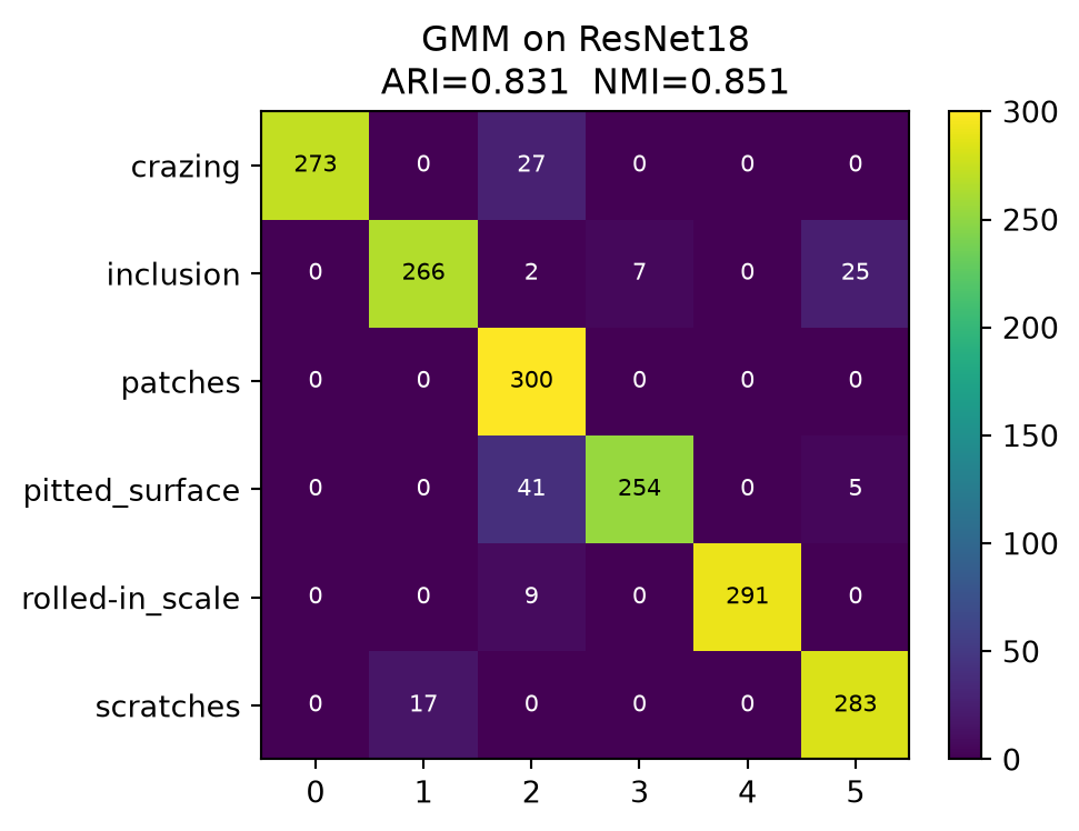
On each we run K-means and a Gaussian Mixture (EM), sweep K, score with ARI / NMI / silhouette / BIC, and visualise with t-SNE + contingency tables.
(adapted from notebooks/MLPC/week05_clustering_neu_det.qmd)
Representation beats algorithm. For both KMeans and GMM, ResNet18 embeddings cluster substantially better than raw-pixel features. The features carry most of the signal; the choice between hard and soft assignment is secondary.
Some defects are easy, others are not. Scratches and patches form visually-coherent clusters; crazing and rolled-in_scale tend to be conflated regardless of features. The contingency heatmaps make this failure mode visible at a glance.
GMM’s soft assignments add interpretability, not accuracy here. Mean assignment entropy is informative (“which samples is the model least sure about?”) but ARI/NMI track KMeans closely.
Block 6 — Reconstruction error as anomaly score
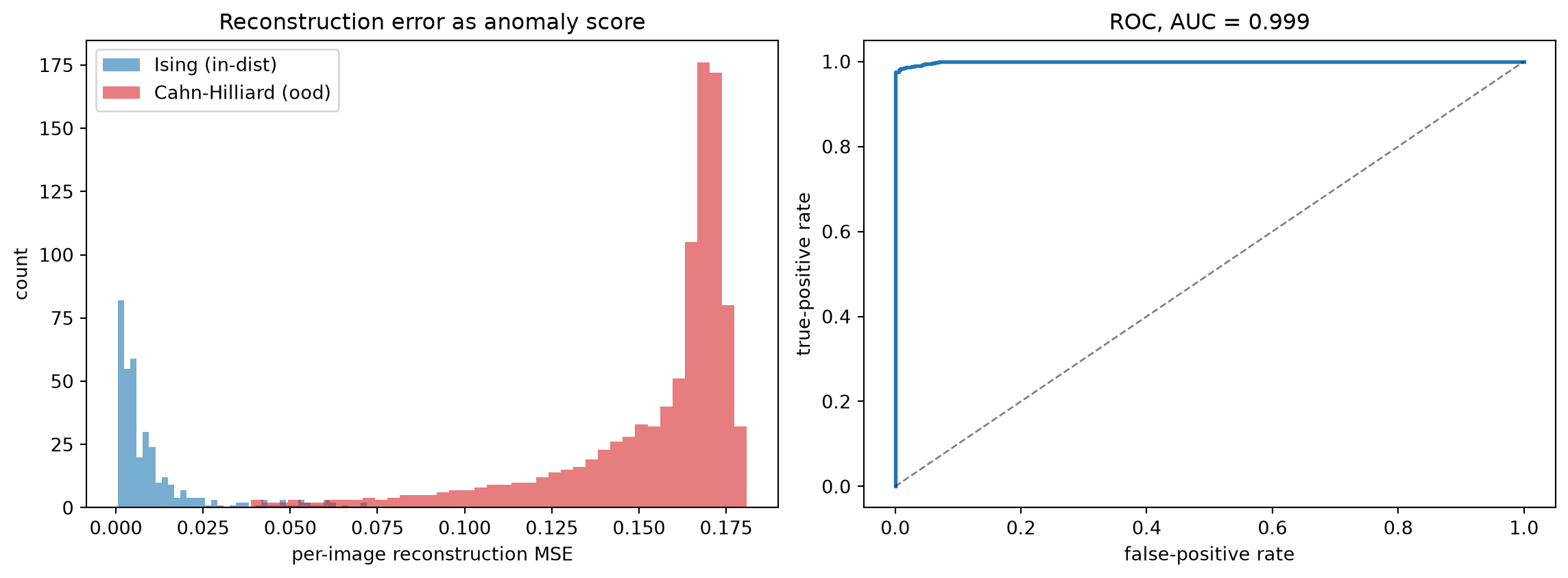
A trained autoencoder reconstructs what it was trained on well, and anything else badly. That is the entire idea behind reconstruction-based anomaly detection: train on “normal” data, score test images by the MSE between input and reconstruction, threshold to flag anomalies.
We score (i) held-out NEU-DET patches (in-distribution — the AE was trained on NEU-DET defects) and (ii) Cahn–Hilliard phase-field snapshots (out-of-distribution — same single-channel grayscale, completely different physics; the loader resizes them to the AE’s 200×200 input on the fly). The reconstruction MSE should separate the two clearly.
(see ML-PC §“Specimen leakage”, §“Reconstruction shortcuts”; MFML §“Denoising autoencoders”)
# In-distribution: held-out NEU-DET val set.def per_image_mse(model, loader, max_n=1000): model.eval() errs = []with torch.no_grad():for x, _ in loader:iftuple(x.shape[-2:]) != AE_IMAGE_SIZE: x = F.interpolate(x, size=AE_IMAGE_SIZE, mode="bilinear", align_corners=False) x = x.to(DEVICE) x_hat = model(x) err = ((x - x_hat) **2).mean(dim=(1, 2, 3)).cpu() # one MSE per image errs.append(err)ifsum(e.numel() for e in errs) >= max_n:breakreturn torch.cat(errs)[:max_n].numpy()id_err = per_image_mse(model, val_loader, max_n=1000)
# Out-of-distribution: a single Cahn-Hilliard simulation as the "anomaly" set.ds_ch = CahnHilliardDataset(simulation_number=0)print(f"Cahn-Hilliard sim 0: N={len(ds_ch)} image shape={tuple(ds_ch.X[0].shape)}")ch_loader = DataLoader(ds_ch, batch_size=256, shuffle=False)ood_err = per_image_mse(model, ch_loader, max_n=1000)# ROC: label 0 = in-distribution Ising, label 1 = out-of-distribution Cahn-Hilliard.y_score = np.concatenate([id_err, ood_err])y_lab = np.concatenate([np.zeros_like(id_err), np.ones_like(ood_err)])auc = roc_auc_score(y_lab, y_score)fpr, tpr, _ = roc_curve(y_lab, y_score)print(f"per-image MSE in-dist median = {np.median(id_err):.4f} ood median = {np.median(ood_err):.4f}")print(f"ROC AUC (Ising vs Cahn-Hilliard, AE trained on Ising) = {auc:.3f}")
Cahn-Hilliard sim 0: N=989   image shape=(1, 64, 64)
per-image MSE   in-dist median = 0.0055   ood median = 0.1660
ROC AUC (Ising vs Cahn-Hilliard, AE trained on Ising) = 0.999
Take-away. Even though Block 5’s latent space did not cleanly separate the six NEU-DET defect classes, the same trained conv-AE still yields a defensible OOD score: the per-image reconstruction MSE histograms for NEU-DET (in-dist) and Cahn–Hilliard (ood) are well separated, and ROC AUC reflects that. One trained model, two unsupervised jobs — and the easier job (OOD detection between two very different physics generators) succeeds even when the harder job (label-recovery clustering) fails. That asymmetry is exactly why MFML and ML-PC both pair clustering with autoencoders in the same unit.
Honest caveat. Distinguishing NEU-DET from Cahn–Hilliard is the easy regime — the two distributions look obviously different to any human, let alone a CNN. Detecting a subtle anomaly inside NEU-DET itself (e.g. a never-seen seventh defect class) is much harder, and is the subject of MFML Unit 11 and ML-PC Unit 10 (Automation in microscopy) later in the semester.
Block 7 — Student exercises
Three core (do all three) + one stretch (optional). Write your code in the empty cells below; bring printed plots / numbers to the next class for the 5-minute walk-through.
Exercise 1 (core) — K-medoids on contaminated nanoindentation
K-means uses the mean as the cluster prototype, which has breakdown point 0: a single outlier can drag the centroid arbitrarily far. K-medoids replaces the mean with an actual data point — the medoid — which gives it robustness to outliers.
Your task:
Take the standardised nanoindentation features from Block 1 (Xn_std, 938 × 2). Inject 5 % synthetic outliers at random by replacing those rows with samples from np.random.normal(loc=10, scale=2) in both features.
Implement K-medoids with the simple PAM-style swap loop below (skeleton given). Run it for K=4 on (a) the clean standardised data and
the contaminated data.
Run K-means on the same two datasets. Report adjusted-Rand index against the original Cr-content labels for all four runs.
Conclusion in two sentences: how much does K-medoids buy you here, and what is the cost in seconds per run?
Hint: the simplest correct PAM implementation alternates an “assign each point to its nearest current medoid” step with a “for each cluster, pick the data point with smallest sum-of-distances to the rest of the cluster as the new medoid” step. ~25 lines.
# YOUR CODE for Exercise 1 below. Skeleton:## def kmedoids(X, K, n_iter=20, rng=None):# rng = rng or np.random.default_rng(0)# # 1. random initial medoids: pick K data indices uniformly# # 2. for each iteration:# # - assignment step: c[i] = argmin_k ||X[i] - X[medoid_k]||# # - update step: new_medoid_k = argmin_{j in C_k} sum_{i in C_k} ||X[i] - X[j]||# # 3. return medoids, assignments# ...
Exercise 2 (core) — Tied-weight autoencoder
A common practical trick: force the decoder weights to be the transpose of the encoder weights. This roughly halves the parameter count and is a soft regulariser (“decoder is the encoder run backwards”).
Your task:
Build a fully-connected tied-weight AE for flattened Ising images with bottleneck \(k=8\):
encoder: z = ReLU(W @ x + b_e) with W of shape (k, d) and d = 4096.
decoder: x_hat = sigmoid(W.T @ z + b_d) (note: same W, transposed).
Train for 3 epochs on flattened Ising-full images using MSE.
Report: parameter count vs the ConvAE from Block 5, and validation MSE.
Hint: subclass nn.Module, store self.W = nn.Parameter(torch.randn(k, d) * 0.01), and call F.linear(x, self.W) for the encoder and F.linear(z, self.W.t()) for the decoder. The two bias parameters are still independent.
# YOUR CODE for Exercise 2 below.
Exercise 3 (core) — Latent-dim sweep (“elbow for autoencoders”)
Just like K-means has an elbow plot for K, autoencoders have one for the latent dimension \(k\). Below a critical \(k\), the bottleneck throws away information the data really needs; above it, you are wasting parameters.
Your task:
Re-train the ConvAE from Block 5 for \(k \in \{1, 2, 4, 8, 16, 32\}\), each for 2 epochs (CPU-friendly).
Record the validation MSE at convergence for each \(k\).
Plot validation MSE vs \(k\). Where is the elbow? Annotate it.
Sanity-check: at \(k = 32\) the AE has more than enough capacity to reconstruct Ising-full. Why is the MSE not (close to) zero?
Hint: write a small train(model, n_epochs) helper to avoid copy-pasting the loop from Block 5 six times.
# YOUR CODE for Exercise 3 below.
Exercise 4 (stretch) — Denoising autoencoder
A denoising AE is trained to reconstruct a clean input from a corrupted version of it. This forces the network to model the manifold the data actually lives on, rather than learning the identity through the bottleneck. Empirically, denoising AEs were the breakthrough that revived autoencoders before VAEs took over (Vincent et al., 2008), and they are the conceptual ancestor of modern diffusion models.
Your task:
Wrap the ConvAE(k=2) architecture in a training loop that, for each batch x, computes x_noisy = (x + 0.3 * torch.randn_like(x)).clamp(0, 1) and trains with loss = MSE(model(x_noisy), x) (target is the clean image).
Train for 5 epochs on Ising-full.
On the held-out validation set, take 5 images, corrupt them with the same noise level, run them through the trained denoising AE, and plot [clean | noisy | reconstruction] triplets.
Compare the latent-space scatter of the denoising AE against the plain AE from Block 5. Is it cleaner / messier / different? Write one sentence interpreting the difference.
# YOUR CODE for Exercise 4 below.
Exam-aligned must-know statements (from MFML Unit 5 §“Exam-aligned”)
Re-read these after the exercises; today’s blocks have given you the concrete intuition for every one of them.
K-means minimises within-cluster variance via Lloyd’s alternating update.
K-means converges to a local minimum; initialisation matters; use k-means++.
K-medoids replaces the mean with an actual data point — robust to outliers, works with any dissimilarity (Exercise 1).
GMMs give soft assignments via responsibilities \(\gamma_{ik}\) (Block 2).
EM alternates an E-step and an M-step; it monotonically increases the log-likelihood (Block 2).
K-means is the limit of GMM with isotropic, equal-variance covariances and zero temperature (Block 3).
PCA = linear encoder + linear decoder + MSE; cannot capture non-linear manifolds (Block 4).
An autoencoder is non-linear encoder/decoder + reconstruction loss; it is self-supervised (Block 5).
A linear autoencoder is equivalent to PCA; non-linear AEs gain power only from the activations (theory bridge between Blocks 4 and 5).
Reconstruction error doubles as an anomaly score for distribution shift (Block 6).