Week 5 — Homework (do BEFORE the Thursday exercise)

This notebook is the mandatory warm-up for the Week 5 in-class exercise. Working through it removes labels from your worldview for an afternoon and gets the K-means mechanics in your fingers, so Thursday can spend its 90 minutes on the harder question: soft assignments and learned latent codes on the same unlabelled microstructure data.

Time: ~85 minutes.

What this homework is

Four short workouts, all anchored on the same idea:

Without labels, the only signal you have is geometry. Distance, density, and reconstruction are the three lenses we will use to read that geometry. K-means is the simplest of the three — it commits to a distance, a number of clusters, and a hard assignment. Everything else we do this week starts by relaxing one of those three commitments.

Part	Min	Topic	Lecture anchor
A	25	Lloyd’s algorithm from scratch on 2-D blobs	MFML §“K-Means as an optimization problem”, §“Lloyd’s algorithm”
B	20	Bad init → local minimum; k-means++; multi-restart; elbow + silhouette	MFML §“Convergence and local minima”, §“Choosing K”
C	30	Standardisation on synthetic (E, H) blobs, then a reality-check on real Cu/Cr nanoindentation	ML-PC §“What unsupervised buys you”, §“Validation problem without labels”
D	10	Reflection: leakage in the unlabelled setting	ML-PC §“Specimen leakage”

What you must hand in (or be able to show on Thursday)

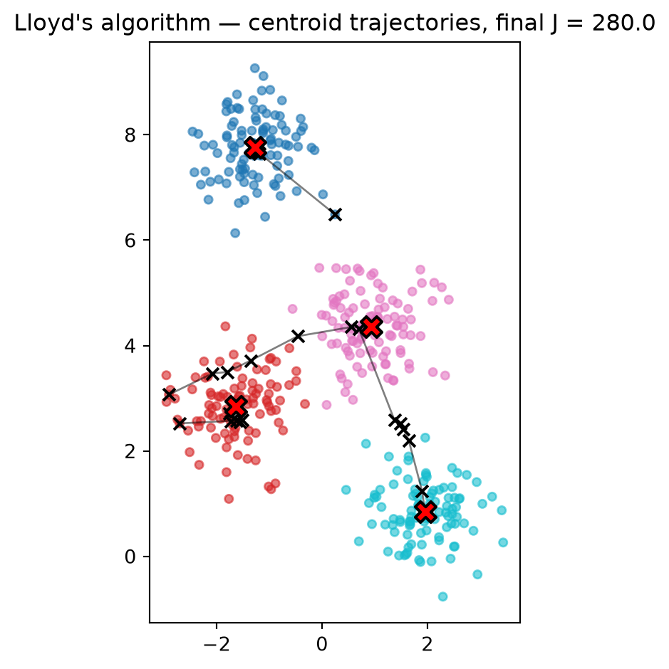
Part A: figure showing centroid trajectories across iterations of your hand-rolled Lloyd loop on the 2-D blobs.
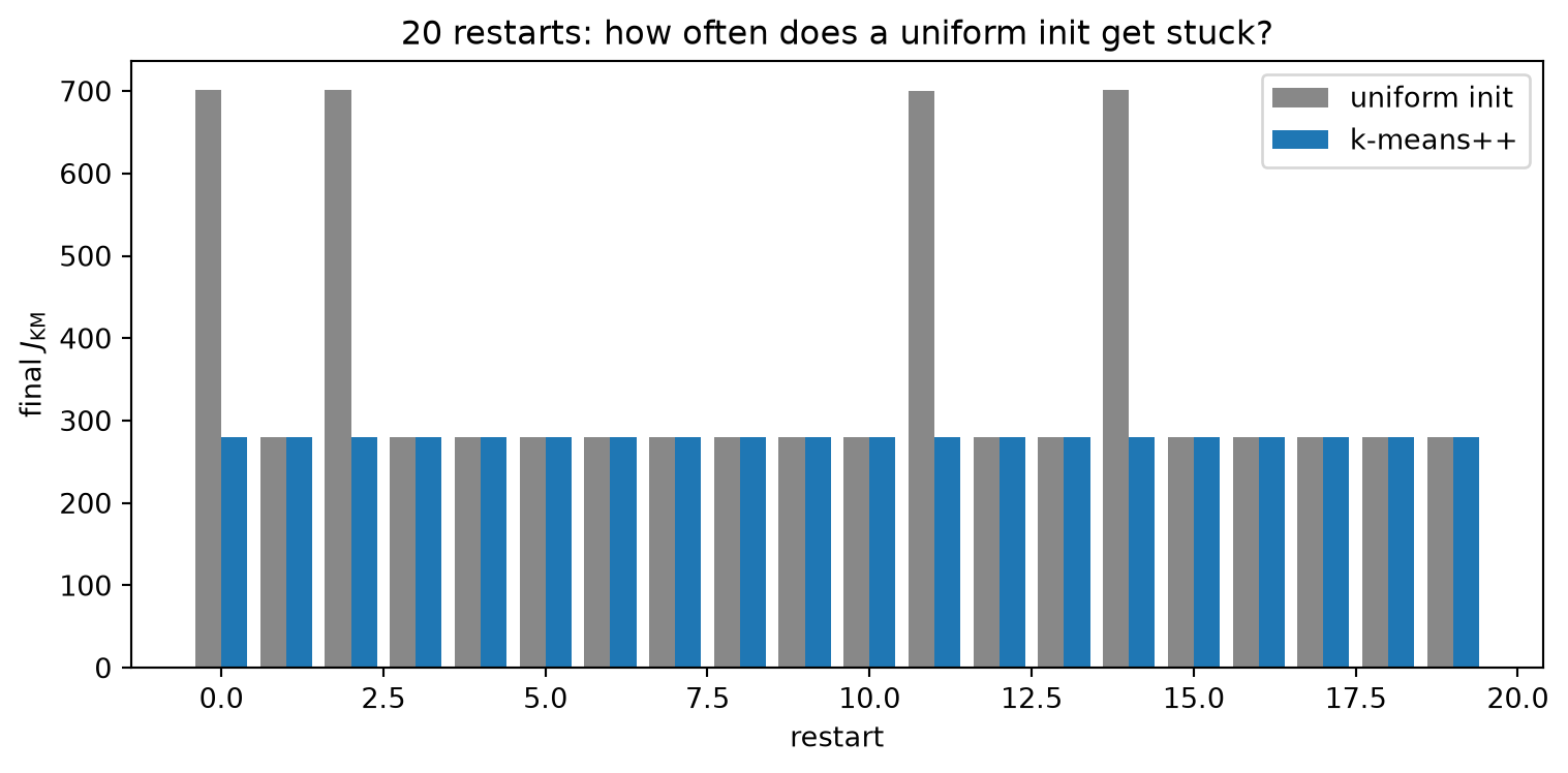
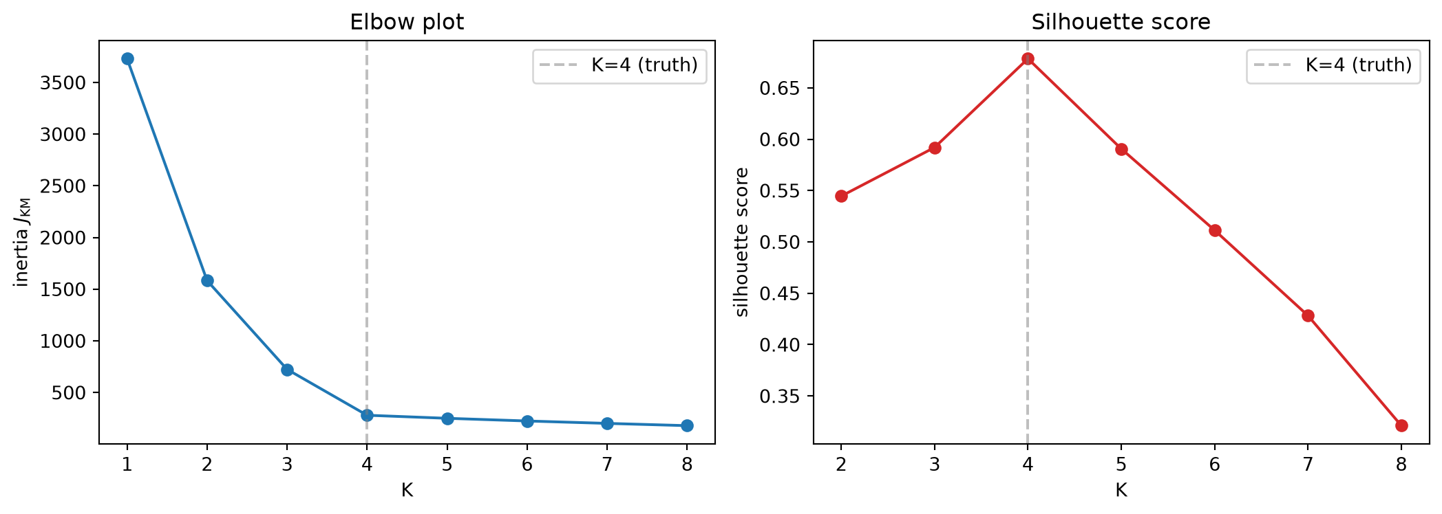
Part B: bar plot of \(J_{\text{KM}}\) across 20 random restarts (uniform init vs k-means++) and an elbow + silhouette plot for K = 1..8.
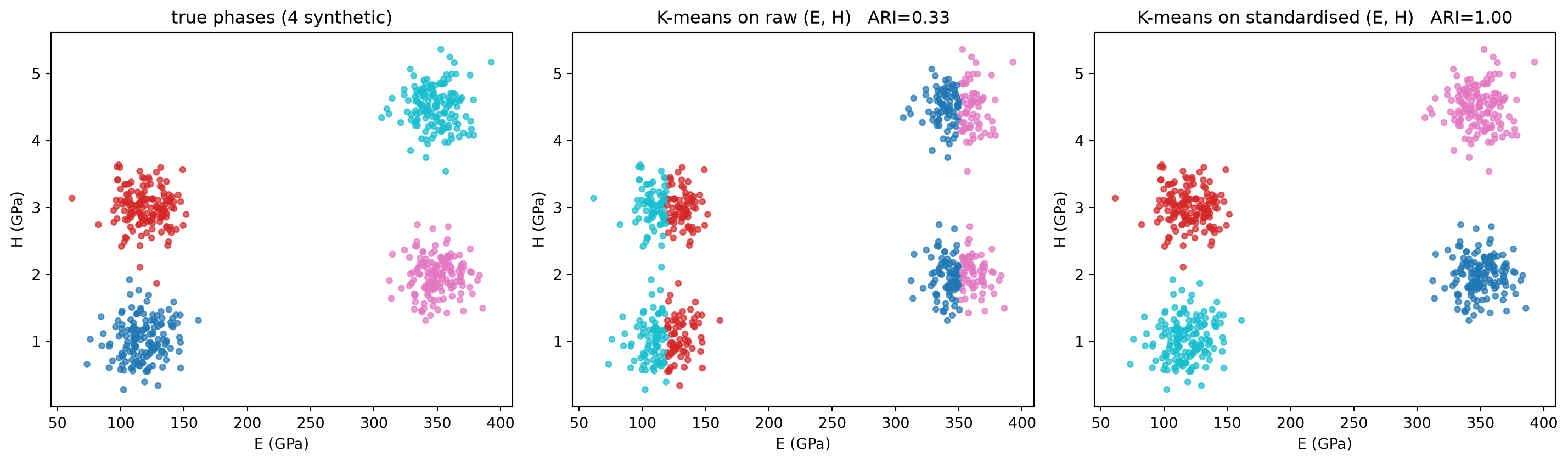
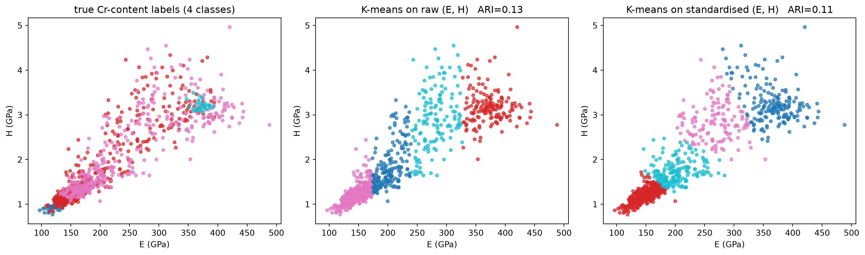
Part C: two three-panel scatters — synthetic (E, H)-like blobs and real nanoindentation — and the four ARI numbers above them; plus one sentence on why standardisation rescues the synthetic case but not the real one.
Part D: your written answer to the leakage reflection (1 paragraph).

# Standard imports for the whole homework. Same idiom as weeks 2-4.
import numpy as np
import torch
import matplotlib.pyplot as plt
from sklearn.datasets import make_blobs
from sklearn.metrics import silhouette_score, adjusted_rand_score

from ai4mat.datasets import NanoindentationDataset

np.random.seed(0)
torch.manual_seed(0)

<torch._C.Generator at 0x7f8605595eb0>

Part A — Lloyd’s algorithm from scratch

We implement K-means in two screens of code so the alternation between “assign every point to its nearest centroid” and “move every centroid to the mean of its points” is visible. Lloyd’s algorithm is two lines of NumPy wrapped in a for loop — there is nothing else to it.

(see MFML §“Lloyd’s algorithm: alternating minimization”)

# A 4-cluster 2-D blob dataset. We keep the ground-truth labels around for
# *evaluation only* — the algorithm never sees them. This mirrors how
# unsupervised methods are validated in practice (slide MFML §"Quality").
X_np, y_true = make_blobs(
    n_samples=400, centers=4, cluster_std=0.6, random_state=0
)
X = torch.tensor(X_np, dtype=torch.float32)
print(f"X shape: {tuple(X.shape)}   true classes: {np.unique(y_true).tolist()}")

X shape: (400, 2)   true classes: [0, 1, 2, 3]

def assign_step(X, mu):
    """E-step analogue: each point joins the nearest centroid.

    X:  (N, d)  data
    mu: (K, d)  centroids
    Returns c: (N,) integer assignment in {0, ..., K-1}.
    """
    # Pairwise squared distances via broadcasting: (N, 1, d) - (1, K, d) -> (N, K, d)
    d2 = ((X[:, None, :] - mu[None, :, :]) ** 2).sum(dim=-1)   # (N, K)
    return d2.argmin(dim=1)


def update_step(X, c, K):
    """M-step analogue: each centroid becomes the mean of its assigned points."""
    return torch.stack([X[c == k].mean(dim=0) for k in range(K)])


def kmeans_objective(X, mu, c):
    """J_KM = sum of squared distances from each point to its assigned centroid."""
    return ((X - mu[c]) ** 2).sum().item()


def lloyd(X, mu_init, n_iter=10):
    """Run Lloyd's algorithm; return the centroid trajectory and per-iter J."""
    K, d = mu_init.shape
    mu = mu_init.clone()
    history = [mu.clone()]
    objective = []
    for _ in range(n_iter):
        c = assign_step(X, mu)
        mu = update_step(X, c, K)
        history.append(mu.clone())
        objective.append(kmeans_objective(X, mu, c))
    return mu, c, torch.stack(history), objective

# Run Lloyd's algorithm with a *deliberately* mediocre initialisation: the
# first 4 data points. This is the classical "uniform random" baseline.
mu0 = X[:4].clone()
mu_final, c_final, history, J_curve = lloyd(X, mu0, n_iter=8)
print(f"final J = {J_curve[-1]:.2f}   monotone decrease? {all(J_curve[i] >= J_curve[i+1] for i in range(len(J_curve)-1))}")

final J = 280.01   monotone decrease? True

# Visualise the centroid trajectory. Each X marker is a centroid at one
# iteration, joined by a line to show how it migrated.
fig, ax = plt.subplots(figsize=(6, 5))
ax.scatter(X[:, 0], X[:, 1], c=c_final, cmap="tab10", s=18, alpha=0.6)
for k in range(4):
    traj = history[:, k, :].numpy()
    ax.plot(traj[:, 0], traj[:, 1], "k-", lw=1, alpha=0.5)
    ax.scatter(traj[:, 0], traj[:, 1], c="k", s=40, marker="x")
    ax.scatter(traj[-1, 0], traj[-1, 1], c="red", s=120, marker="X",
               edgecolors="k", linewidths=1.5, zorder=5)
ax.set_title(f"Lloyd's algorithm — centroid trajectories, final J = {J_curve[-1]:.1f}")
ax.set_aspect("equal")
plt.tight_layout()
plt.show()

Part A deliverable: the figure above. Notice that every centroid moves a lot in iteration 1, very little by iteration 4, and not at all by the end — this is the monotone-decrease guarantee of Lloyd’s algorithm in action.

Part B — Initialisation, k-means++, and choosing K

Lloyd’s algorithm only finds a local minimum of \(J_{\text{KM}}\), and the local minimum it finds depends entirely on the initial centroids. Two practical fixes: (i) run from many random starts and keep the best, and (ii) initialise smartly with k-means++, which spreads the initial centroids out by sampling proportional to squared distance from already chosen ones.

(see MFML §“Convergence and local minima”, §“Smarter initialization — k-means++”)

def kmeanspp_init(X, K, rng):
    """k-means++ initialisation. Each new centroid is sampled with
    probability proportional to D(x)^2, the squared distance to the
    nearest already-chosen centroid (Arthur & Vassilvitskii, 2007)."""
    N = X.shape[0]
    # First centroid: pick uniformly at random from the data.
    idx0 = int(rng.integers(N))
    centers = [X[idx0]]
    for _ in range(K - 1):
        mu_so_far = torch.stack(centers)            # (k_chosen, d)
        d2 = ((X[:, None, :] - mu_so_far[None, :, :]) ** 2).sum(dim=-1)
        d2_min = d2.min(dim=1).values               # (N,) nearest existing centroid
        probs = (d2_min / d2_min.sum()).numpy()
        idx = int(rng.choice(N, p=probs))
        centers.append(X[idx])
    return torch.stack(centers)

# Compare 20 restarts of (i) uniform random init vs (ii) k-means++ init.
# Same data, same Lloyd loop, only the initialisation differs.
n_restarts = 20
J_uniform, J_kpp = [], []
rng = np.random.default_rng(0)
for r in range(n_restarts):
    # Uniform: pick K random data points.
    idx = rng.choice(len(X), size=4, replace=False)
    mu0_u = X[idx].clone()
    _, c_u, _, J_u = lloyd(X, mu0_u, n_iter=15)
    J_uniform.append(J_u[-1])

    # k-means++.
    mu0_p = kmeanspp_init(X, K=4, rng=rng)
    _, c_p, _, J_p = lloyd(X, mu0_p, n_iter=15)
    J_kpp.append(J_p[-1])

print(f"uniform  init: J min = {min(J_uniform):.1f}   J max = {max(J_uniform):.1f}   J mean = {np.mean(J_uniform):.1f}")
print(f"k-means++    : J min = {min(J_kpp):.1f}   J max = {max(J_kpp):.1f}   J mean = {np.mean(J_kpp):.1f}")

uniform  init: J min = 280.0   J max = 701.8   J mean = 364.2
k-means++    : J min = 280.0   J max = 280.0   J mean = 280.0

# Bar plot of the 20 final-J values. The spread of the uniform bars *is*
# the local-minimum problem; the k-means++ bars are tighter and lower.
fig, ax = plt.subplots(figsize=(8, 4))
width = 0.4
xs = np.arange(n_restarts)
ax.bar(xs - width / 2, J_uniform, width, label="uniform init", color="#888888")
ax.bar(xs + width / 2, J_kpp,     width, label="k-means++",   color="#1f77b4")
ax.set_xlabel("restart"); ax.set_ylabel("final $J_{\\mathrm{KM}}$")
ax.set_title("20 restarts: how often does a uniform init get stuck?")
ax.legend()
plt.tight_layout()
plt.show()

# Choosing K: elbow + silhouette. We use sklearn here because the point is
# the *diagnostic*, not another implementation of Lloyd. We range K = 1..8.
from sklearn.cluster import KMeans

K_range = list(range(1, 9))
inertia = []
silhouette = []
for K in K_range:
    km = KMeans(n_clusters=K, n_init=10, random_state=0).fit(X_np)
    inertia.append(km.inertia_)
    if K >= 2:
        silhouette.append(silhouette_score(X_np, km.labels_))
    else:
        silhouette.append(np.nan)   # silhouette undefined for K=1

fig, axes = plt.subplots(1, 2, figsize=(11, 4))
axes[0].plot(K_range, inertia, "o-"); axes[0].set_xlabel("K"); axes[0].set_ylabel("inertia $J_{\\mathrm{KM}}$")
axes[0].set_title("Elbow plot")
axes[1].plot(K_range, silhouette, "o-", color="#d62728"); axes[1].set_xlabel("K"); axes[1].set_ylabel("silhouette score")
axes[1].set_title("Silhouette score")
for ax in axes:
    ax.axvline(4, color="gray", ls="--", alpha=0.5, label="K=4 (truth)")
    ax.legend(loc="best")
plt.tight_layout()
plt.show()

Part B deliverables: the bar plot and the elbow+silhouette plot. The silhouette curve in particular should peak right at K=4 — this is the only diagnostic in this notebook that actually picks K rather than just describing it.

Part C — When standardisation matters: a synthetic-then-real story

Two short subsections, one lesson, one cliffhanger.

C.1 (synthetic, ~10 min): the cleanest possible demonstration of why standardisation matters when features have different units.
C.2 (real, ~20 min): the same recipe on real Cu/Cr nanoindentation data — and a confrontation with the limits of what K-means can recover when the labels you care about aren’t in the features you have.

(see ML-PC §“What unsupervised buys you”, §“Validation problem without labels”)

C.1 — Synthetic blobs in (E, H)-like units

Imagine four hypothetical alloy phases. Two of them share a Young’s modulus of ~120 GPa and two share ~350 GPa; within each E-pair, the phases differ only in hardness \(H\). This is the geometric configuration where raw-feature K-means is forced to fail: the inter-cluster gap in \(E\) (~230 GPa) dwarfs the inter-cluster gap in \(H\) (~2 GPa), so raw Euclidean distance is essentially “distance in \(E\)”, and the \(H\)-split is invisible.

# Four synthetic phases. Two pairs share an E centre and differ only in H.
rng_syn = np.random.default_rng(0)
centers = np.array([
    [120.0, 1.0],   # phase 0: low E, soft
    [120.0, 3.0],   # phase 1: low E, hard       — same E as phase 0
    [350.0, 2.0],   # phase 2: high E, soft
    [350.0, 4.5],   # phase 3: high E, very hard — same E as phase 2
])
stds = np.array([15.0, 0.3])    # E-spread is ~50x H-spread, like real (E, H)
n_per = 150

X_syn = np.concatenate([
    centers[k] + stds * rng_syn.standard_normal((n_per, 2))
    for k in range(4)
])
y_syn = np.repeat(np.arange(4), n_per)
print(f"synthetic: N={len(X_syn)}   "
      f"E in [{X_syn[:, 0].min():.0f}, {X_syn[:, 0].max():.0f}] GPa   "
      f"H in [{X_syn[:, 1].min():.2f}, {X_syn[:, 1].max():.2f}] GPa")

synthetic: N=600   E in [62, 393] GPa   H in [0.28, 5.36] GPa

# K-means on RAW vs STANDARDISED. Same algorithm, same K, only scaling differs.
km_syn_raw = KMeans(n_clusters=4, n_init=10, random_state=0).fit(X_syn)

mu_syn, sd_syn = X_syn.mean(axis=0), X_syn.std(axis=0)
X_syn_s = (X_syn - mu_syn) / sd_syn
km_syn_std = KMeans(n_clusters=4, n_init=10, random_state=0).fit(X_syn_s)

ari_syn_raw = adjusted_rand_score(y_syn, km_syn_raw.labels_)
ari_syn_std = adjusted_rand_score(y_syn, km_syn_std.labels_)
print(f"synthetic, RAW          features: ARI vs phase labels = {ari_syn_raw:.3f}")
print(f"synthetic, STANDARDISED features: ARI vs phase labels = {ari_syn_std:.3f}")

synthetic, RAW          features: ARI vs phase labels = 0.333
synthetic, STANDARDISED features: ARI vs phase labels = 0.996

# Three-panel comparison on the synthetic data.
fig, axes = plt.subplots(1, 3, figsize=(15, 4.5))
for ax, c, title in zip(
    axes,
    [y_syn, km_syn_raw.labels_, km_syn_std.labels_],
    ["true phases (4 synthetic)",
     f"K-means on raw (E, H)   ARI={ari_syn_raw:.2f}",
     f"K-means on standardised (E, H)   ARI={ari_syn_std:.2f}"],
):
    ax.scatter(X_syn[:, 0], X_syn[:, 1], c=c, cmap="tab10", s=14, alpha=0.7)
    ax.set_xlabel("E (GPa)"); ax.set_ylabel("H (GPa)"); ax.set_title(title)
plt.tight_layout()
plt.show()

What you should see. Raw K-means slices the data along the \(E\) axis only — the 230 GPa gap between phase-pairs dwarfs the 2 GPa \(H\)-gap, so phases 0/1 (both at \(E\!\approx\!120\)) are merged and phases 2/3 (both at \(E\!\approx\!350\)) are merged. The “extra” two clusters are spent splitting each \(E\)-mode along \(E\) itself, because that’s where the variance lives in raw units. Standardisation puts \(E\) and \(H\) on equal footing, the \(H\)-split becomes legible to the algorithm, and ARI jumps from ~0.3 to ≈1.0.

This is the standardisation lesson, full stop: when features have different units, raw Euclidean distance is a fiction — K-means is effectively clustering on whichever feature has the largest numerical range.

C.2 — Real Cu/Cr nanoindentation: same recipe, harder reality

Now the same pipeline on real data. The NanoindentationDataset contains 938 measurements of Young’s modulus \(E\) (GPa) and hardness \(H\) (GPa) on Cu/Cr composites with four nominal Cr-content levels (0 / 25 / 60 / 100 %). The labels exist for evaluation only — the metallurgist’s day-to-day question is “are there really four regimes in this batch, and which specimen lands in which?”.

Critical caveat before you run anything: in C.1 we designed the labels to be present in the (E, H) geometry. Real labels are a different story, and what happens next is the reason Thursday’s session exists.

ds = NanoindentationDataset()
Xn = ds.X.numpy()                      # (938, 2)
yn = ds.y.numpy()                      # (938,)  with 4 classes
print(f"Nanoindentation: N={len(ds)}   features=(E [GPa], H [GPa])   classes={np.unique(yn).tolist()}")
print(f"raw ranges:  E in [{Xn[:, 0].min():.1f}, {Xn[:, 0].max():.1f}]   H in [{Xn[:, 1].min():.2f}, {Xn[:, 1].max():.2f}]")

Nanoindentation: N=938   features=(E [GPa], H [GPa])   classes=[0, 1, 2, 3]
raw ranges:  E in [96.7, 488.2]   H in [0.77, 4.96]

# K-means on RAW vs STANDARDISED. Identical recipe to C.1.
km_raw  = KMeans(n_clusters=4, n_init=10, random_state=0).fit(Xn)

mu_, sd_ = Xn.mean(axis=0), Xn.std(axis=0)
Xs = (Xn - mu_) / sd_
km_std = KMeans(n_clusters=4, n_init=10, random_state=0).fit(Xs)

ari_raw = adjusted_rand_score(yn, km_raw.labels_)
ari_std = adjusted_rand_score(yn, km_std.labels_)
print(f"K-means on RAW          features:  ARI vs Cr-content labels = {ari_raw:.3f}")
print(f"K-means on STANDARDISED features:  ARI vs Cr-content labels = {ari_std:.3f}")

K-means on RAW          features:  ARI vs Cr-content labels = 0.128
K-means on STANDARDISED features:  ARI vs Cr-content labels = 0.111

# Three-panel comparison: ground truth, raw-feature K-means, standardised K-means.
fig, axes = plt.subplots(1, 3, figsize=(15, 4.5))
for ax, c, title in zip(
    axes,
    [yn, km_raw.labels_, km_std.labels_],
    [f"true Cr-content labels (4 classes)",
     f"K-means on raw (E, H)   ARI={ari_raw:.2f}",
     f"K-means on standardised (E, H)   ARI={ari_std:.2f}"],
):
    ax.scatter(Xn[:, 0], Xn[:, 1], c=c, cmap="tab10", s=14, alpha=0.7)
    ax.set_xlabel("E (GPa)"); ax.set_ylabel("H (GPa)"); ax.set_title(title)
plt.tight_layout()
plt.show()

What you should see — and why C.1 was a controlled lie. Both ARI numbers are mediocre (around 0.1) and standardisation barely moves the needle. The reason is structural, not a bug:

The true labels (left panel) form a continuous diagonal manifold in \((E, H)\). All four Cr-content classes overlap heavily; the 25 % and 60 % populations are essentially inseparable, and the 100 % Cr cluster is buried inside the others near the origin.
K-means does find four clean clusters in this data — they just aren’t the Cr-content labels. They are the four geometric regimes the \((E, H)\) scatter actually contains.

This is the failure mode the lecture spent time on: clustering recovers geometry, not semantics. When the labels you care about don’t live in your features, no amount of algorithmic sophistication can conjure them. Standardisation didn’t fail — it did its job (compare the cluster geometry between the raw and standardised panels: vertical bands vs diagonal regimes), the data just doesn’t carry the Cr-content signal in two dimensions.

Thursday’s question. What do we actually do when K-means on the features we have cannot recover the labels we want? Thursday explores three answers in sequence:

Relax the assignment — soft, probabilistic membership via GMM/EM, and the realisation that K-means is just GMM with frozen, isotropic, \(\sigma^2\!\to\!0\) covariances (Blocks 2–3).
Change the representation — on a different materials dataset (NEU-DET steel-surface defects) where the labels do live in the pixels, we compare a linear baseline (PCA) against a non-linear autoencoder and pretrained image features (Blocks 4–5).
Change the question — use the trained autoencoder’s reconstruction error as an anomaly score instead of chasing semantic labels (Block 6).

The C.2 result above is the warning shot for all of these: when geometry and semantics disagree, no clustering algorithm rescues you on its own — feature engineering and problem framing do.

Part C deliverables:

The synthetic three-panel scatter (C.1) with its two ARI numbers — showing the big gap between raw and standardised.
The real-nanoindentation three-panel scatter (C.2) with its two ARI numbers — showing the small gap, and a Cr-content scatter that clearly doesn’t separate into four blobs.
One sentence in your own words: why standardisation rescued the synthetic case but not the real one.

Part D — Reflection: leakage in the unlabelled setting

In Week 3 we hammered the rule “split before you preprocess; split by specimen, not by sample”. You may be tempted to believe that unsupervised methods are immune to leakage because there is no train/test split and no labels to leak.

They are not. Two ways leakage still bites:

Specimen / replicate leakage in K selection. If you pick K by silhouette on a dataset that contains 100 patches from each of 50 specimens, the silhouette is dominated by within-specimen similarity — the algorithm “discovers” the specimens, not the phases. The fix is to score silhouette on a held-out specimen set or to aggregate measurements per specimen first.
Standardisation across a future test set. If you standardise using statistics computed on a pool that includes a future sample, you have silently encoded knowledge of that sample into the clustering. The fix is the same as in supervised learning: fit the scaler on the training pool only, then transform the rest.

Your task (~10 min, write 4–6 sentences): Take one of the two leakage modes above, and describe how you would detect it in your own data — what plot or metric would change if leakage is present versus absent? Bring this paragraph to Thursday; we will pick two volunteers to read theirs aloud at the start of Block 1.

Hand in: your written paragraph (Markdown cell below).

(your reflection paragraph here)