Week 6 — Homework (do BEFORE the Thursday exercise)
This notebook is the mandatory warm-up for the Week 6 in-class exercise. It puts the optimizer toolkit from MFML Unit 6 in your fingers and the composition-only descriptor baseline from MG Unit 6 in your training loop, so Thursday’s 90 minutes can spend itself on the integrated story: fine-tuning across phase fields (ML-PC Unit 6) and graph-aware regression on crystals (MG Unit 5).
Time: ~75 minutes.
Red thread
The optimizer is one toolbox. The same SGD/momentum/Adam choices apply whether the input is a synthetic 2-D bowl, an Ising microstructure image, or a 4-feature element vector. Today you build optimizer intuition on toy losses (Part A), watch it on a real CNN (Part B), and then watch it again on a tiny materials regressor (Part C). Thursday we will keep the optimizer toolkit fixed and change the input — fine-tuning across phase fields and message-passing on crystal graphs.
What this homework is
Part
Min
Topic
Lecture anchor
A
25
Hand-rolled SGD, momentum, Adam on three 2-D losses
What you must hand in (or be able to show on Thursday)
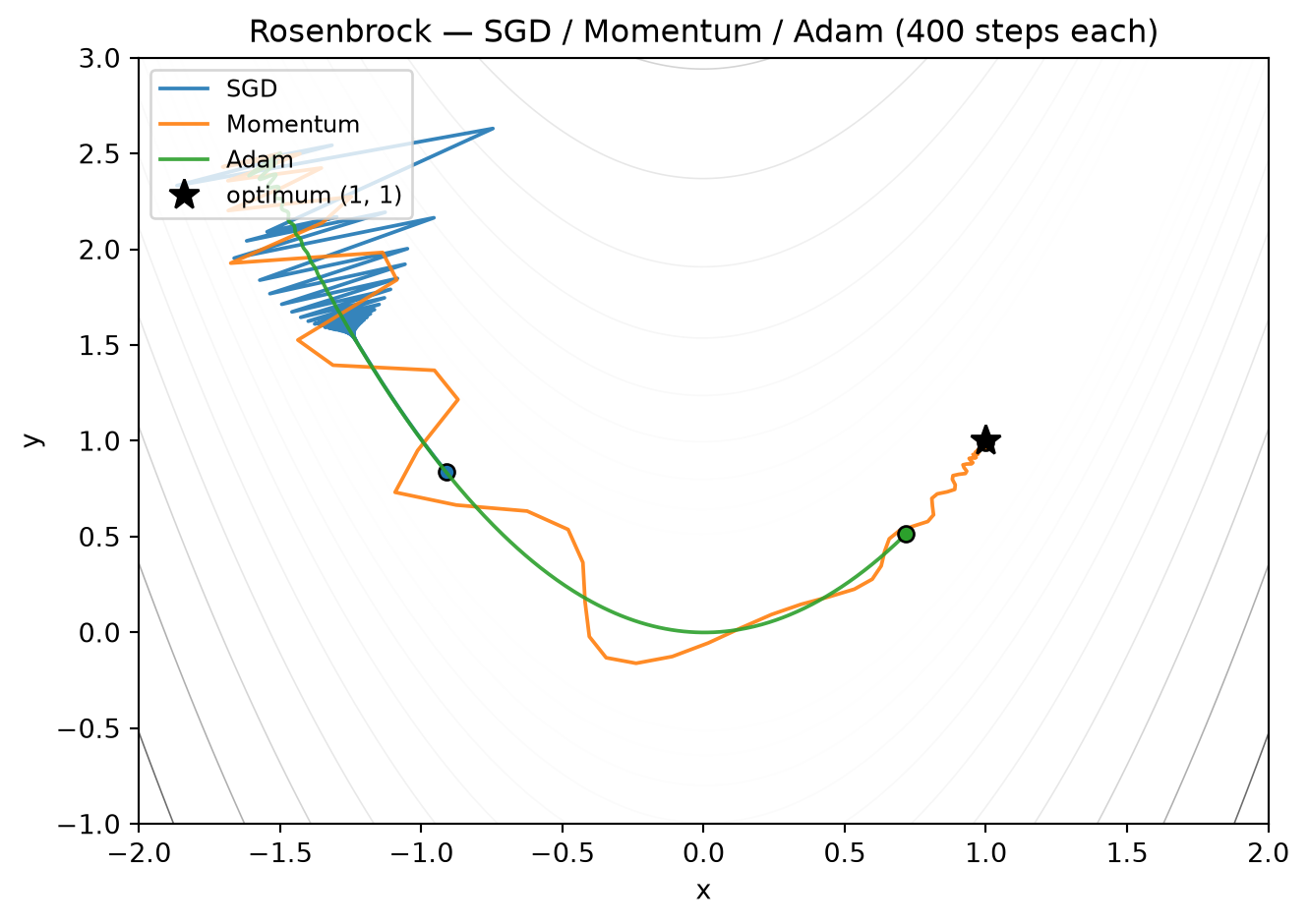
Part A: side-by-side trajectory plot for SGD vs momentum vs Adam on the Rosenbrock function.
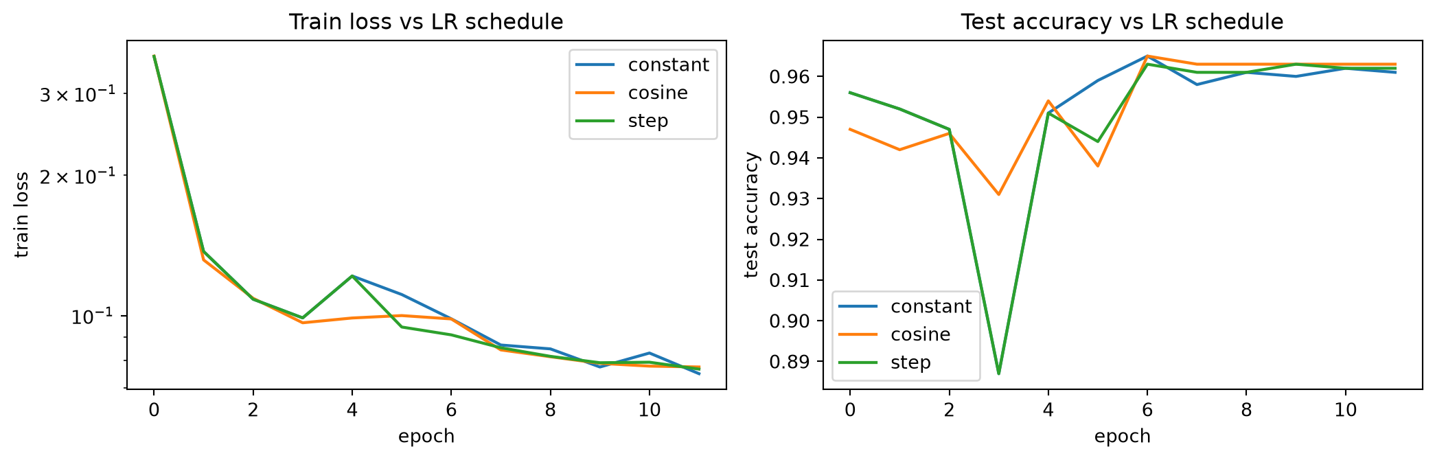
Part B: overlaid loss curves for constant / cosine / step LR schedules on the Ising-light CNN; printed final-epoch test accuracy per schedule.
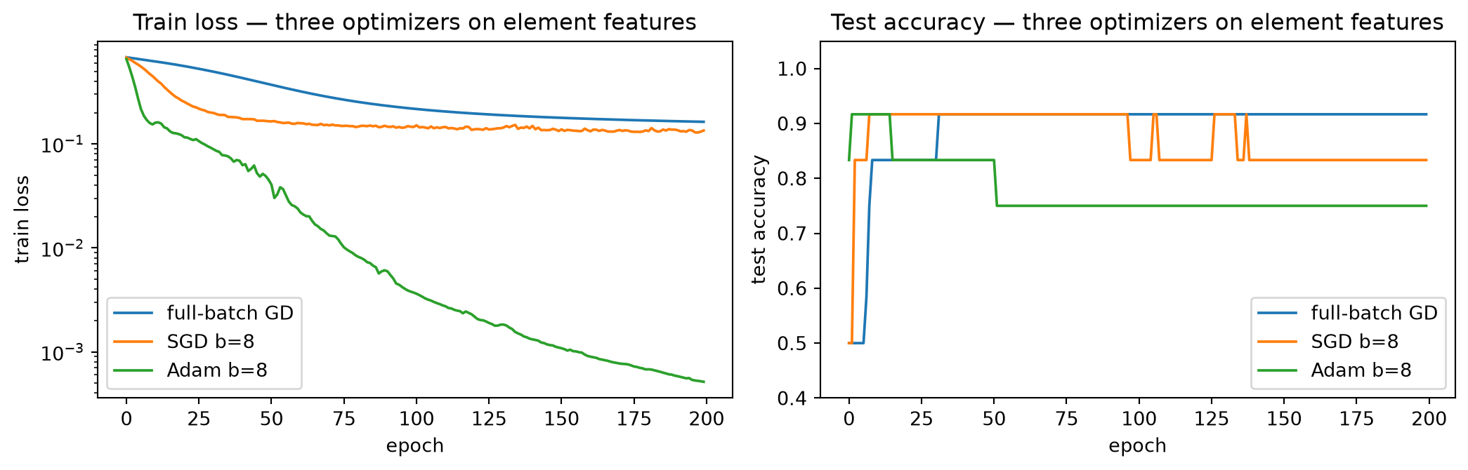
Part C: training and test curves for the three optimizer presets on ChemicalElementsDataset; printed final test accuracy table.
Part D: your written paragraph (~5 sentences).
# Standard imports for the whole homework. Same idiom as weeks 2-5.import mathimport numpy as npimport torchimport torch.nn as nnimport torch.nn.functional as Ffrom torch.utils.data import DataLoader, random_splitimport matplotlib.pyplot as pltfrom ai4mat.datasets import IsingDataset, ChemicalElementsDatasetnp.random.seed(0)torch.manual_seed(0)
<torch._C.Generator at 0x7fe2dc1cddf0>
Part A — Optimizer playground on 2-D losses
We hand-roll three optimizers — vanilla SGD, SGD + momentum, and Adam — and watch them navigate three pathological 2-D landscapes:
A stretched ravine: \(f(x, y) = 10 x^2 + 0.1 y^2\). The condition number is 100; SGD bounces, Adam normalizes per-axis steps.
The Rosenbrock banana, \(f(x, y) = (1 - x)^2 + 100(y - x^2)^2\), a classic stress test for first-order methods.
We implement the optimizers in plain PyTorch so you can see exactly what each one does. The point is not to beat torch.optim; it is to read the update rules.
(see MFML §“Vanilla SGD”, §“Momentum: the heavy ball”, §“Adam — RMSProp plus bias-corrected momentum”)
def sgd_step(x, grad, lr, state):"""Vanilla stochastic gradient descent: x <- x - lr * grad."""return x - lr * grad, statedef momentum_step(x, grad, lr, state, beta=0.9):"""SGD + momentum (heavy ball): v <- beta v + grad; x <- x - lr * v.""" v = state.get("v", torch.zeros_like(x)) v = beta * v + grad state["v"] = vreturn x - lr * v, statedef adam_step(x, grad, lr, state, beta1=0.9, beta2=0.999, eps=1e-8):"""Adam: per-parameter LR via running mean (m) and variance (v).""" m = state.get("m", torch.zeros_like(x)) v = state.get("v", torch.zeros_like(x)) t = state.get("t", 0) +1 m = beta1 * m + (1- beta1) * grad v = beta2 * v + (1- beta2) * grad **2 m_hat = m / (1- beta1 ** t) v_hat = v / (1- beta2 ** t) state.update(m=m, v=v, t=t)return x - lr * m_hat / (torch.sqrt(v_hat) + eps), statedef run_optimizer(x0, grad_fn, step_fn, lr, n_iter):"""Run any of the above for `n_iter` steps; return the trajectory.""" x = x0.clone().detach().requires_grad_(False) state = {} traj = [x.clone()]for _ inrange(n_iter): grad = grad_fn(x) x, state = step_fn(x, grad, lr, state) traj.append(x.clone())return torch.stack(traj)
# Three loss functions and their hand-coded gradients.def saddle_grad(x):return torch.tensor([2.0* x[0], -2.0* x[1]])def ravine_grad(x):return torch.tensor([20.0* x[0], 0.2* x[1]])def rosenbrock_grad(x): a, b =1.0, 100.0 dx =-2* (a - x[0]) -4* b * x[0] * (x[1] - x[0] **2) dy =2* b * (x[1] - x[0] **2)return torch.tensor([dx, dy])
# Run all three optimizers on the Rosenbrock banana. Tune the LRs to make# each optimizer competitive — Rosenbrock punishes a too-large step size.x0 = torch.tensor([-1.5, 2.5])traj_sgd = run_optimizer(x0, rosenbrock_grad, sgd_step, lr=0.0013, n_iter=400)traj_mom = run_optimizer(x0, rosenbrock_grad, momentum_step, lr=0.0014, n_iter=400)traj_adam = run_optimizer(x0, rosenbrock_grad, adam_step, lr=0.09, n_iter=400)# Plot the loss landscape with all three trajectories overlaid.xs = torch.linspace(-2, 2, 200)ys = torch.linspace(-1, 3, 200)XX, YY = torch.meshgrid(xs, ys, indexing="xy")Z = (1- XX) **2+100* (YY - XX **2) **2fig, ax = plt.subplots(figsize=(7, 5))ax.contour(XX, YY, Z, levels=np.logspace(-1, 3.5, 25), cmap="Greys", linewidths=0.6)for traj, label, color in [ (traj_sgd, "SGD", "C0"), (traj_mom, "Momentum", "C1"), (traj_adam, "Adam", "C2"),]: ax.plot(traj[:, 0], traj[:, 1], "-", color=color, lw=1.4, label=label, alpha=0.9) ax.plot(traj[-1, 0], traj[-1, 1], "o", color=color, mec="k", ms=6)ax.plot(1, 1, "k*", ms=12, label="optimum (1, 1)")ax.set_title("Rosenbrock — SGD / Momentum / Adam (400 steps each)")ax.set_xlabel("x"); ax.set_ylabel("y"); ax.legend(loc="upper left", fontsize=9)plt.tight_layout(); plt.show()
What you should see on the Rosenbrock plot. SGD crawls along the narrow valley floor and stops well short of (1, 1) within 400 steps. Momentum builds velocity along the valley axis and gets much closer. Adam normalizes the step per-axis — its trajectory looks straighter than the other two.
Try yourself (optional but recommended): rerun the cell above with saddle_grad and ravine_grad and a starting point of [-1.0, 1.0]. On the saddle, vanilla SGD stalls near the origin; momentum and Adam both escape but in qualitatively different ways. On the ravine, SGD with the same LR will diverge along the steep axis — that’s the ill-conditioning story from MFML §“Why the LR has to be conservative”.
Part A.4 — Visualizing Lion’s sign-of-gradient update
The three optimizers above (SGD / momentum / Adam) are the classic trio. Since Chen et al. 2023 [@chen_2023_lion] the modern alternative Lion has gained adoption: instead of normalizing the update by a running estimate of variance (Adam) or by adapting the step size in any continuous way, Lion takes the sign of a momentum-smoothed gradient. The update magnitude is constant per axis — only the sign changes.
That sounds drastic, so let us see it on the classic ill-conditioned quadratic
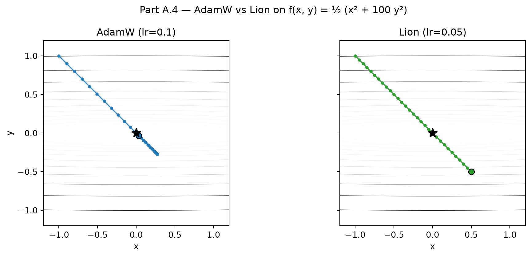
The Hessian eigenvalues are 1 and 100; the loss is a long, narrow valley. We start at \((x_0, y_0) = (-1, 1)\) and run 50 steps each of AdamW (using torch.optim) and a hand-rolled Lion that we write in five lines. We plot the trajectories side by side.
def lion_step(x, grad, lr, state, beta1=0.9, beta2=0.99):"""Lion: u = sign(beta1 * m + (1 - beta1) * grad); x <- x - lr * u. The momentum buffer is updated AFTER the parameter step (Chen et al. 2023 convention). The point of this cell is that the *magnitude* of the update along each axis is exactly `lr` — only the sign changes. """ m = state.get("m", torch.zeros_like(x)) u = torch.sign(beta1 * m + (1.0- beta1) * grad) x_new = x - lr * u m = beta2 * m + (1.0- beta2) * grad state["m"] = mreturn x_new, statedef ill_quad_grad(x):return torch.tensor([x[0], 100.0* x[1]])
# Run AdamW for 50 steps starting at (-1, 1). We use torch.optim.AdamW on# a single leaf-tensor parameter so the trajectory is honest.torch.manual_seed(0)x0 = torch.tensor([-1.0, 1.0])n_iter =30p = torch.nn.Parameter(x0.clone())adamw = torch.optim.AdamW([p], lr=0.1, weight_decay=0.0)traj_adamw = [p.detach().clone()]for _ inrange(n_iter): adamw.zero_grad() loss =0.5* (p[0] **2+100.0* p[1] **2) loss.backward() adamw.step() traj_adamw.append(p.detach().clone())traj_adamw = torch.stack(traj_adamw)# Hand-rolled Lion from the same start; smaller LR because Lion's update# magnitude is constant (= lr) per axis.traj_lion = run_optimizer(x0, ill_quad_grad, lion_step, lr=0.05, n_iter=n_iter)
Reading the side-by-side plot. The AdamW trajectory is smooth — its update magnitudes shrink continuously as the running variance estimates climb along the steep (\(y\)) axis. The Lion trajectory is visibly staircased: each step moves by exactly lr along the sign of the (momentum-smoothed) gradient, so the optimizer makes large constant strides early and then cannot shrink them when it gets close to the minimum. That is the central trade-off Lion makes: by giving up the variance estimate (saving one tensor of optimizer state per parameter), it also gives up the ability to taper its step size.
Instructor note. This is why Lion needs a smaller LR than AdamW in practice — the update magnitude is lr per axis, not lr times a small adaptive factor. The rule of thumb in the literature is 3-10× smaller than the AdamW LR you would otherwise use. Show this plot before the Block 5 bake-off in the Thursday lecture so the LR-grid choice (Lion sweeps {3e-4, 1e-3, 3e-3} vs AdamW’s {3e-3, 1e-2, 3e-2}) is motivated rather than mysterious.
Forward link: see the MFML W6 slide deck, “Modern alternatives to AdamW (2023–2024)” — Lion, Sophia, Schedule-Free AdamW.
Part B — LR schedules on a 2-conv CNN
Now we put the optimizer choice inside a real training loop. The model is a tiny 2-conv CNN trained on IsingDataset(size='light') (16×16 microstructure images, 5000 samples, binary Curie-temperature classification). The point is not to set a record on Ising — that problem is easy — it is to compare three LR schedules on the same model and the same data, with everything else held fixed.
Three schedules:
Constant — the naïve baseline.
Cosine annealing — LR decays from lr_max to ~0 along a cosine curve over the full training run. The MFML W6 default for fine-tuning.
Step decay — LR halves at epoch 5 and again at epoch 10. Common in older image-classification recipes.
(see MFML §“Cosine annealing”, §“Step decay”, §“How LR interacts with batch size”)
# Model + data setup. Three identical CNNs (one per schedule), trained on# the same data, same batch size, same total epochs.class TinyCNN(nn.Module):def__init__(self, n_classes=2):super().__init__()self.conv1 = nn.Conv2d(1, 8, kernel_size=3, padding=1)self.conv2 = nn.Conv2d(8, 16, kernel_size=3, padding=1)self.pool = nn.MaxPool2d(2)self.fc = nn.Linear(16*4*4, n_classes)def forward(self, x): x =self.pool(F.relu(self.conv1(x))) x =self.pool(F.relu(self.conv2(x)))returnself.fc(x.flatten(1))ising = IsingDataset(size="light")n_train =int(0.8*len(ising))train_ds, test_ds = random_split( ising, [n_train, len(ising) - n_train], generator=torch.Generator().manual_seed(0),)train_loader = DataLoader(train_ds, batch_size=64, shuffle=True)test_loader = DataLoader(test_ds, batch_size=256)print(f"Ising-light: {len(train_ds)} train, {len(test_ds)} test")
Ising-light: 4000 train, 1000 test
# Schedule definitions: each one is a function step -> LR.N_EPOCHS =12N_STEPS = N_EPOCHS *len(train_loader)LR_MAX =0.03def schedule_constant(step):return LR_MAXdef schedule_cosine(step): frac = step / N_STEPSreturn0.5* LR_MAX * (1+ math.cos(math.pi * frac))def schedule_step(step): epoch = step //len(train_loader)if epoch <5:return LR_MAXelif epoch <10:return LR_MAX /2.0else:return LR_MAX /4.0
def train_one(schedule_fn, label):"""Train a fresh TinyCNN under the given LR schedule. Returns curves.""" torch.manual_seed(0) model = TinyCNN() optim_ = torch.optim.SGD(model.parameters(), lr=LR_MAX, momentum=0.9) train_loss, test_acc = [], [] step =0for epoch inrange(N_EPOCHS): model.train() running =0.0for xb, yb in train_loader:for g in optim_.param_groups: g["lr"] = schedule_fn(step) optim_.zero_grad() loss = F.cross_entropy(model(xb), yb) loss.backward() optim_.step() running += loss.item() * xb.shape[0] step +=1 train_loss.append(running /len(train_ds)) model.eval() n_correct =0with torch.no_grad():for xb, yb in test_loader: n_correct += (model(xb).argmax(1) == yb).sum().item() test_acc.append(n_correct /len(test_ds))print(f" {label:9s} final test acc = {test_acc[-1]:.3f}")return train_loss, test_accprint("Training three schedules:")loss_const, acc_const = train_one(schedule_constant, "constant")loss_cos, acc_cos = train_one(schedule_cosine, "cosine")loss_step, acc_step = train_one(schedule_step, "step")
Training three schedules:
  constant   final test acc = 0.961
  cosine     final test acc = 0.963
  step       final test acc = 0.962
# Plot loss curves and test accuracy side-by-side.fig, (ax1, ax2) = plt.subplots(1, 2, figsize=(11, 3.6))for losses, label, c in [(loss_const, "constant", "C0"), (loss_cos, "cosine", "C1"), (loss_step, "step", "C2")]: ax1.plot(losses, "-", color=c, label=label, lw=1.6)ax1.set_xlabel("epoch"); ax1.set_ylabel("train loss"); ax1.set_yscale("log")ax1.set_title("Train loss vs LR schedule"); ax1.legend()for accs, label, c in [(acc_const, "constant", "C0"), (acc_cos, "cosine", "C1"), (acc_step, "step", "C2")]: ax2.plot(accs, "-", color=c, label=label, lw=1.6)ax2.set_xlabel("epoch"); ax2.set_ylabel("test accuracy")ax2.set_title("Test accuracy vs LR schedule"); ax2.legend()plt.tight_layout(); plt.show()
What the LR-schedule plot tells you. The constant LR keeps making big steps even when the loss has flattened — final-epoch loss sits well above the cosine and step variants. Cosine and step both anneal toward the end of training; the cosine curve is smoother because the schedule itself is smooth. On Ising-light the test-accuracy gap is small (the task is easy); on harder problems the gap can be 1–3 percentage points.
Repeat with Adam (optional). Swap torch.optim.SGD for torch.optim.Adam and rerun. You’ll typically see Adam reach a worse minimum faster — this is the ML-PC W6 anti-pattern that we’ll hit again on Thursday in Block 5.
Part C — Optimizer choice on ChemicalElementsDataset
Now we leave the image domain and train a tiny materials regressor on ChemicalElementsDataset: 38 elements × 4 features (atomic radius, electron affinity, ionization energy, electronegativity), task is binary metallic-vs-nonmetallic.
This is the simplest rung of MG Unit 6’s descriptor ladder: composition-only features that don’t even need a structure. The dataset is small enough that we can do full-batch gradient descent by hand and read every gradient step. We then compare to:
SGD with batch size 8 — same model, same LR, but minibatched.
Adam — adaptive per-parameter step.
(see MG §“The descriptor ladder”, §“Magpie elemental statistics”, §“Why composition-only descriptors are stronger than they should be”; ML-PC §“Optimization recap”)
elements = ChemicalElementsDataset()X, y = elements.X, elements.y # (38, 4), (38,)X = (X - X.mean(0)) / X.std(0) # standardiseprint(f"X shape: {tuple(X.shape)} y shape: {tuple(y.shape)} y mean: {y.mean():.3f}")# 70/30 train/test split, fixed seed.g = torch.Generator().manual_seed(0)perm = torch.randperm(len(X), generator=g)n_tr =int(0.7*len(X))tr, te = perm[:n_tr], perm[n_tr:]X_tr, y_tr = X[tr], y[tr]X_te, y_te = X[te], y[te]
X shape: (38, 4) y shape: (38,) y mean: 0.579
class TinyMLP(nn.Module):"""4 -> 16 -> 16 -> 1 with ReLUs. Output is a single logit."""def__init__(self):super().__init__()self.net = nn.Sequential( nn.Linear(4, 16), nn.ReLU(), nn.Linear(16, 16), nn.ReLU(), nn.Linear(16, 1), )def forward(self, x):returnself.net(x).squeeze(-1)def accuracy(model, Xb, yb):with torch.no_grad():return ((torch.sigmoid(model(Xb)) >0.5).float() == yb).float().mean().item()def train_mlp(optimizer_factory, label, n_epochs=200, batch_size=None):"""Train one TinyMLP with the given optimizer; return loss + acc curves. If batch_size is None, train full-batch GD. Else SGD with the given batch size (single-pass shuffled minibatches). """ torch.manual_seed(0) model = TinyMLP() optim_ = optimizer_factory(model.parameters()) losses, train_accs, test_accs = [], [], []for ep inrange(n_epochs): model.train()if batch_size isNone: optim_.zero_grad() loss = F.binary_cross_entropy_with_logits(model(X_tr), y_tr) loss.backward() optim_.step()else: perm_b = torch.randperm(len(X_tr)) running =0.0for i inrange(0, len(X_tr), batch_size): idx = perm_b[i:i + batch_size] optim_.zero_grad() loss = F.binary_cross_entropy_with_logits(model(X_tr[idx]), y_tr[idx]) loss.backward() optim_.step() running += loss.item() * idx.numel() loss = torch.tensor(running /len(X_tr)) losses.append(loss.item()) train_accs.append(accuracy(model, X_tr, y_tr)) test_accs.append(accuracy(model, X_te, y_te))print(f" {label:24s} final test acc = {test_accs[-1]:.3f}")return np.array(losses), np.array(train_accs), np.array(test_accs)
# Three optimizer presets. Same model, same data, same epochs, same seed;# only the optimizer differs.print("Training three optimizer presets on ChemicalElementsDataset:")loss_gd, acc_tr_gd, acc_te_gd = train_mlp(lambda p: torch.optim.SGD(p, lr=0.05),"full-batch GD (lr=0.05)", batch_size=None,)loss_sgd, acc_tr_sgd, acc_te_sgd = train_mlp(lambda p: torch.optim.SGD(p, lr=0.05),"SGD batch=8 (lr=0.05)", batch_size=8,)loss_ad, acc_tr_ad, acc_te_ad = train_mlp(lambda p: torch.optim.Adam(p, lr=0.01),"Adam batch=8 (lr=0.01)", batch_size=8,)
Training three optimizer presets on ChemicalElementsDataset:
  full-batch GD (lr=0.05)   final test acc = 0.917
  SGD batch=8 (lr=0.05)     final test acc = 0.833
  Adam batch=8 (lr=0.01)    final test acc = 0.750
# Plot side-by-side.fig, (ax1, ax2) = plt.subplots(1, 2, figsize=(11, 3.6))for losses, label, c in [(loss_gd, "full-batch GD", "C0"), (loss_sgd, "SGD b=8", "C1"), (loss_ad, "Adam b=8", "C2")]: ax1.plot(losses, "-", color=c, label=label, lw=1.4)ax1.set_xlabel("epoch"); ax1.set_ylabel("train loss"); ax1.set_yscale("log")ax1.set_title("Train loss — three optimizers on element features"); ax1.legend()for accs, label, c in [(acc_te_gd, "full-batch GD", "C0"), (acc_te_sgd, "SGD b=8", "C1"), (acc_te_ad, "Adam b=8", "C2")]: ax2.plot(accs, "-", color=c, label=label, lw=1.4)ax2.set_xlabel("epoch"); ax2.set_ylabel("test accuracy"); ax2.set_ylim(0.4, 1.05)ax2.set_title("Test accuracy — three optimizers on element features"); ax2.legend()plt.tight_layout(); plt.show()
Final-epoch test accuracy (write this down for Thursday):
optimizer
batch
test acc
full-batch GD
full
%.3f
SGD
8
%.3f
Adam
8
%.3f
(Numbers will be filled in when you run the cell above.)
What this small experiment shows.
On a 4-feature problem with 27 training examples, not all three optimizers converge to a comparable accuracy in the end. The descriptor ladder’s bottom rung — composition-only features — is strong on this task.
Full-batch GD is the smoothest curve (no minibatch noise).
SGD with batch 8 wiggles more but reaches almost the same place.
This is the “implicit prior” view: the descriptor (4-vector of element properties) carries most of the information; the optimizer’s job is to find the bias-variance trade-off, not to discover the features. Thursday’s GNN will learn its own per-element features from a graph — and we’ll watch the optimizer’s job get harder as the input gets richer.
Part D — Reflection (1 paragraph, ~5 sentences)
Write a paragraph answering: when does Adam help, and when does it hurt? Specifically, comment on:
small-batch vs full-batch training,
ill-conditioned losses (very different curvature along different axes),
fine-tuning a pretrained model.
Reference one observation from your Part A trajectories and one from your Part C accuracy table.
Bridge to Thursday. On Thursday we’ll train a CNN on Ising and then fine-tune it on Cahn–Hilliard. The classical result you’ll see: Adam with the same LR you used for the source task wrecks fine-tuning; SGD with momentum + a cosine schedule recovers it. Your Part D paragraph should already have an opinion about why.
You’re done with Week 6 homework. Bring your four deliverables on Thursday:
Rosenbrock trajectory plot (Part A).
LR-schedule loss curves on Ising-light (Part B).
Optimizer-preset accuracy table on ChemicalElementsDataset (Part C).