This week we braid three lectures around a single decision: what does the optimizer do?
MFML Unit 6: Optimization for deep learning — SGD, momentum, Adam, ill-conditioning, learning-rate schedules, batch effects.
ML-PC Unit 6: Transfer learning as continued optimization on a related loss landscape — catastrophic forgetting, discriminative LRs, cosine schedules + warm-up, why Adam often hurts during fine-tuning.
MG Unit 6: Local atomic environments — the descriptor ladder (composition → RDF → coordination → SOAP) and universal ML interatomic potentials as pretrained backbones you fine-tune.
Red thread:The optimizer is one toolbox. Today we apply it to two inputs — a 64×64 phase-field image being fine-tuned across distributions (Ising → Cahn–Hilliard) and a frozen SOAP local-environment fingerprint regressed with a small head. A fixed descriptor is a frozen backbone and a universal MLIP is a pretrained one — so the MG modality is the same linear-probe / fine-tune story, with atoms as the input.
Pre-flight check. This notebook assumes you have run notebooks/week6_homework.py. Block 1 picks up directly from your Part A trajectories and Part C optimizer table; we will not re-derive them.
Agenda (90 min)
Block
Min
Topic
1
~6
Recap from homework — optimizer trajectories + element baseline
2
~14
Catastrophic forgetting: Ising → Cahn–Hilliard with too-high LR
3
~12
Discriminative learning rates: backbone vs head
4
~14
Cosine schedule + warm-up rescues fine-tuning
5
~12
Modern optimizer bake-off — AdamW vs Adam+L2 vs Lion vs Schedule-Free AdamW
6
~18
MG W6: SOAP local environments + universal MLIPs (frozen-backbone braid)
7
~22
Student exercises (3 core + 1 stretch)
# Standard imports. Same idiom as weeks 2-5: explicit seeds, no hidden state.import mathimport copyimport numpy as npimport torchimport torch.nn as nnimport torch.nn.functional as Ffrom torch.utils.data import DataLoader, random_split, Subsetimport matplotlib.pyplot as pltfrom ai4mat.datasets import ( IsingDataset, CahnHilliardDataset,)np.random.seed(0)torch.manual_seed(0)
<torch._C.Generator at 0x7f69cffee710>
Helpers used by every block
We use the same CNN backbone as in homework Part B but at 64×64 (Ising full, not light) so it has enough capacity to be interesting under fine-tuning. The architecture has two halves — a convolutional backbone and a small head. The split lets us freeze, unfreeze, and re-LR each half independently.
Two takeaways from the homework that frame the rest of the lecture:
From Part A (Rosenbrock): vanilla SGD crawls; momentum builds velocity along the valley axis; Adam normalizes the step per axis.
From Part C (ChemicalElementsDataset): on a 4-feature regressor with ~27 training examples, all three optimizers reach roughly the same accuracy. The descriptor (composition-only, MG U6 ladder bottom rung) carries the signal. The optimizer’s job was easy.
Today the optimizer’s job will not be easy. Two ways the input gets harder: (a) the loss landscape changes when we fine-tune (Blocks 2–5); (b) the input is a frozen SOAP local-environment fingerprint, not a 4-vector or an image — a fixed pretrained representation (Block 6).
# Build a *source-task* CNN: Ising-full classification, trained from scratch# in ~30 seconds on CPU. We will reuse this exact set of weights as the# starting point for every fine-tuning experiment in Blocks 2-5.ising = IsingDataset(size="full")n_train =int(0.8*len(ising))ising_train, ising_test = random_split( ising, [n_train, len(ising) - n_train], generator=torch.Generator().manual_seed(0),)ising_train_loader = DataLoader(ising_train, batch_size=64, shuffle=True)ising_test_loader = DataLoader(ising_test, batch_size=256)torch.manual_seed(0)source_model = CNN(n_classes=2)optim_ = torch.optim.SGD(source_model.parameters(), lr=0.03, momentum=0.9)print("Pretraining source model on Ising-full (3 epochs, ~30 s on CPU)...")for epoch inrange(3): source_model.train()for xb, yb in ising_train_loader: optim_.zero_grad() F.cross_entropy(source_model(xb), yb).backward() optim_.step()print(f" source-task test acc on Ising-full: {evaluate(source_model, ising_test_loader):.3f}")# Freeze a deep copy of the trained weights so every fine-tuning experiment# starts from the *exact same* initialization. This is the moral equivalent# of loading a checkpoint.SOURCE_STATE = copy.deepcopy(source_model.state_dict())
Pretraining source model on Ising-full (3 epochs, ~30 s on CPU)...
  source-task test acc on Ising-full: 0.991
# Build a *target-task* dataset: Cahn-Hilliard with the free energy# binarised at its median. 64x64 grayscale, two classes — same shape and# task type as Ising, but a *different* generative process. This is the# "related but not identical" distribution shift that makes fine-tuning# well-defined.print("Loading Cahn-Hilliard (3 simulations, ~3000 samples)...")ch_full = CahnHilliardDataset(simulation_number=[0, 1, 2])print(f" loaded {len(ch_full)} samples; energy range = [{ch_full.y.min():.3g}, {ch_full.y.max():.3g}]")ch_y_bin = (ch_full.y > ch_full.y.median()).long()class CahnHilliardBinary(torch.utils.data.Dataset):def__init__(self, base, y_bin, idx):self.base = baseself.y_bin = y_binself.idx = idxdef__len__(self):returnlen(self.idx)def__getitem__(self, i): j =int(self.idx[i])returnself.base.X[j], self.y_bin[j]# Use a small subset (1500 train, 500 test) for fast iteration during the lecture.g = torch.Generator().manual_seed(0)perm = torch.randperm(len(ch_full), generator=g)[:2000]ch_train_idx, ch_test_idx = perm[:1500], perm[1500:2000]ch_train = CahnHilliardBinary(ch_full, ch_y_bin, ch_train_idx)ch_test = CahnHilliardBinary(ch_full, ch_y_bin, ch_test_idx)ch_train_loader = DataLoader(ch_train, batch_size=64, shuffle=True)ch_test_loader = DataLoader(ch_test, batch_size=256)print(f" fine-tuning subset: {len(ch_train)} train, {len(ch_test)} test")
  loaded 2975 samples; energy range = [458, 1.1e+03]
  fine-tuning subset: 1500 train, 500 test
Block 2 — Catastrophic forgetting under uniform LR
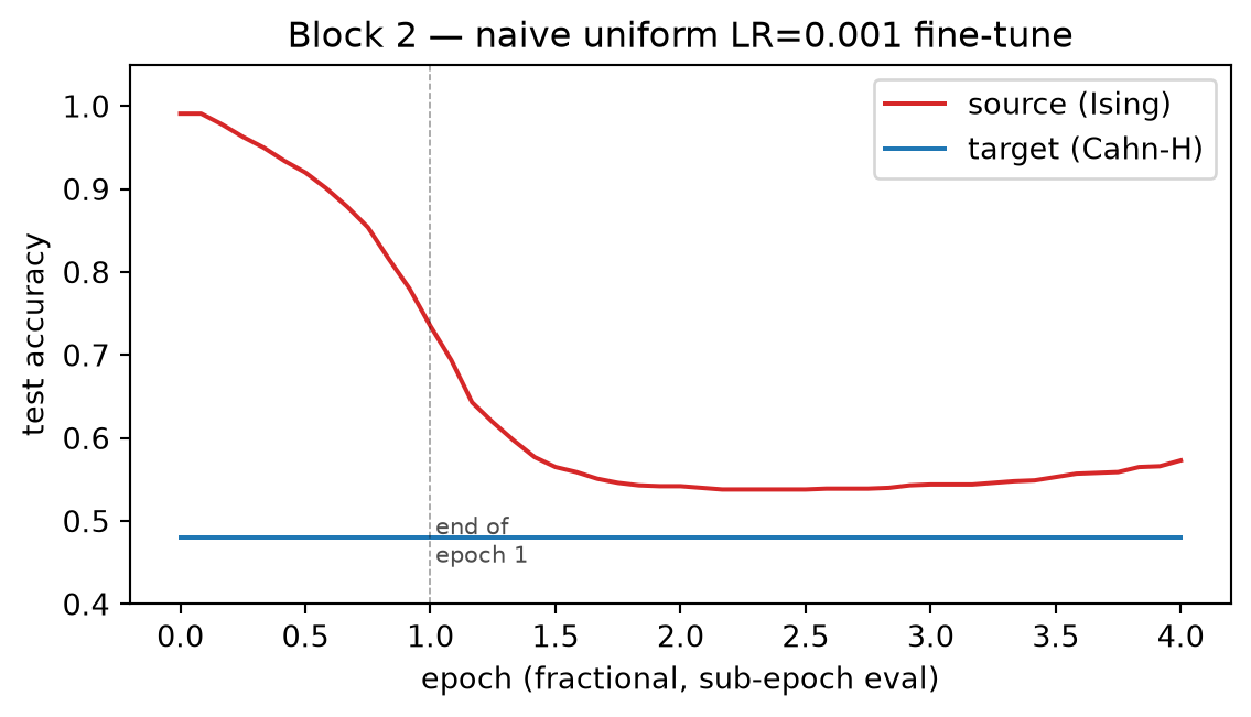
Naive transfer learning recipe: load source weights, train on the target task with a single uniform LR for backbone and head — no schedule, no discriminative-LR trick. We watch both test accuracies — source (Ising) and target (Cahn-Hilliard) — across the fine-tune.
Two things make this block subtle. First, the collapse happens inside the first epoch (≈24 batches) at any LR that lets the target task learn at all, so we evaluate every two batches, not once per epoch — a per-epoch probe just records “both at 0.5” and misses the actual trajectory. Second, the LR we pick (1e-3) is not outrageous; it is exactly the “small uniform LR” comparison Block 3 will run. The punchline: even a modest uniform LR is catastrophic for the source task. From the optimizer’s point of view this is SGD on a non-stationary loss — yesterday’s loss is forgotten as soon as today’s gradient overwrites it.
(see ML-PC §“Catastrophic forgetting = SGD on a non-stationary loss”, §“Why fine-tuning needs careful optimization”)
def fine_tune(state_dict, lr_backbone, lr_head, n_epochs=4, optimizer_cls=torch.optim.SGD, scheduler=None, freeze_backbone=False, momentum=0.9, eval_every_batches=None):"""Fine-tune source weights on Cahn-Hilliard. Track BOTH accuracies. Index 0 of the returned arrays is always the *initial* measurement (before any training step), so per-epoch arrays have length ``n_epochs + 1``. Pass ``eval_every_batches=k`` to measure every ``k`` training batches instead — Block 2 uses this to resolve the catastrophic-forgetting trajectory, which collapses *inside* a single epoch and is invisible to a once-per-epoch probe. """ torch.manual_seed(0) model = CNN(n_classes=2) model.load_state_dict(state_dict)if freeze_backbone:for p in model.backbone.parameters(): p.requires_grad =False param_groups = [{"params": model.head.parameters(), "lr": lr_head}]else: param_groups = [ {"params": model.backbone.parameters(), "lr": lr_backbone}, {"params": model.head.parameters(), "lr": lr_head}, ]if optimizer_cls is torch.optim.SGD: optim_ = optimizer_cls(param_groups, momentum=momentum)else: optim_ = optimizer_cls(param_groups) sched = scheduler(optim_) if scheduler isnotNoneelseNone src_acc = [evaluate(model, ising_test_loader)] tgt_acc = [evaluate(model, ch_test_loader)] step =0for ep inrange(n_epochs): model.train()for xb, yb in ch_train_loader:# Update LR for *this* step before optim_.step(). Calling# sched.step() AFTER optim_.step() (the more common PyTorch# idiom) would leave the very first batch at the optimizer's# initial lr_max — a silent off-by-one that defeats warm-up# entirely and blasts the source basin on the *first* gradient# update.if sched isnotNone: sched.step() optim_.zero_grad() F.cross_entropy(model(xb), yb).backward() optim_.step() step +=1if eval_every_batches isnotNoneand step % eval_every_batches ==0: src_acc.append(evaluate(model, ising_test_loader)) tgt_acc.append(evaluate(model, ch_test_loader))if eval_every_batches isNone: src_acc.append(evaluate(model, ising_test_loader)) tgt_acc.append(evaluate(model, ch_test_loader))return np.array(src_acc), np.array(tgt_acc)
Reading the plot. Source accuracy starts at ~0.99 (the Ising checkpoint) and decays smoothly to chance (~0.51) over the first ~10 batches as the Ising-trained head and backbone are re-aligned by Cahn-Hilliard gradients. Target accuracy stays near chance during this re-alignment (the head is being rotated, not yet aimed at the new labels), then climbs over epochs 2–4 to ≈0.95. The dashed line marks the end of epoch 1 — note that the entire source collapse happens to the left of it, which is why a per-epoch probe would just read “0.5 everywhere” and miss the catastrophe.
The key point is not that the LR is too high — 1e-3 is the same value Block 3 uses as the “small uniform LR” comparison. The point is that uniform-LR fine-tuning has no mechanism to preserve source knowledge: the optimizer minimizes today’s loss with whatever weights it can move, and the head is the most movable thing in the network.
Two ways out — both standard ML-PC W6 fixes — explored next.
Block 3 — Discriminative learning rates
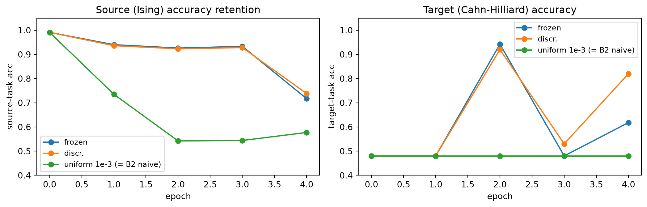
Classical recipe (ULMFiT, Howard & Ruder 2018): lower LR on the backbone than on the head, because the backbone already knows something useful (Ising textures = Cahn-Hilliard textures, roughly) and only needs fine refinement; the head is fresh and can take big steps. We compare three protocols at the same total budget:
Frozen backbone — head only, LR 1e-2.
Discriminative LRs — backbone 1e-4, head 1e-2 (factor 100).
Full unfreezing at uniform LR — same LR everywhere, 1e-3. This is the Block 2 naive baseline at per-epoch resolution, kept in the comparison as a foil — we already know it forgets the source.
(see ML-PC §“Layer-wise / discriminative learning rates”)
Block 3 — three protocols at fixed budget:
  frozen backbone:        source=0.717  target=0.618
  discriminative LRs:     source=0.738  target=0.820
  uniform LR (small):     source=0.577  target=0.480
# Per-epoch plots include the initial (epoch 0) state, so arrays have# length n_epochs + 1. "uniform 1e-3" here is the same configuration# Block 2 used as the naive baseline — Block 2 just measured it at# sub-epoch resolution to expose the in-epoch collapse.fig, (a1, a2) = plt.subplots(1, 2, figsize=(11, 3.6))ep = np.arange(len(src_frozen))for src, label, c in [(src_frozen, "frozen", "C0"), (src_disc, "discr.", "C1"), (src_uni, "uniform 1e-3 (= B2 naive)", "C2")]: a1.plot(ep, src, "o-", label=label, c=c)a1.set_title("Source (Ising) accuracy retention")a1.set_xlabel("epoch"); a1.set_ylabel("source-task acc")a1.set_ylim(0.4, 1.05); a1.legend(fontsize=9)for tgt, label, c in [(tgt_frozen, "frozen", "C0"), (tgt_disc, "discr.", "C1"), (tgt_uni, "uniform 1e-3 (= B2 naive)", "C2")]: a2.plot(ep, tgt, "o-", label=label, c=c)a2.set_title("Target (Cahn-Hilliard) accuracy")a2.set_xlabel("epoch"); a2.set_ylabel("target-task acc")a2.set_ylim(0.4, 1.05); a2.legend(fontsize=9)plt.tight_layout(); plt.show()
Reading the comparison. Frozen backbone keeps the source-task features intact (we never touched the conv weights), so source acc stays well above chance even though the head was retrained on Cahn-Hilliard labels. Discriminative LRs do at least as well on source retention and let the target task improve past the frozen ceiling, because the backbone can still nudge toward the new distribution. The uniform-LR foil reaches a high target accuracy but pays for it by collapsing the source to chance — exactly the catastrophe Block 2 dissected at sub-epoch resolution.
Take-home. Discriminative LRs are an implementation of the prior we want: “the backbone is approximately right; nudge it; the head is fresh; train it normally.” A uniform LR is unable to express that prior at any single value — too small and nothing learns, too large (which here means anything ≥ 1e-3) and the source is gone.
The naive Block-2 collapse came from one decision: constant LR at the source-task value. The fix is mechanical, not magical: anneal the LR along a cosine, with a short warm-up at the start so the optimizer does not take a huge first step into a fresh head.
(see MFML §“Cosine annealing”, §“Warm-up”, ML-PC §“Cosine schedules / warm-up for fine-tuning”)
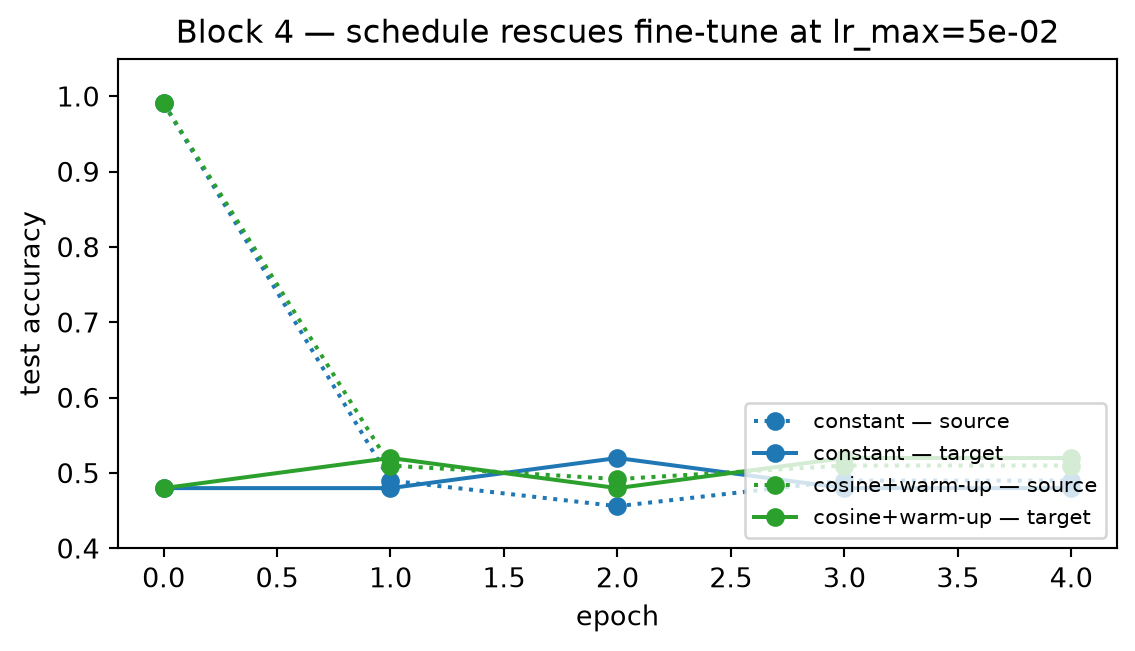
def cosine_with_warmup(optim_, n_warmup_steps, n_total_steps, lr_max_per_group):"""Custom step-level scheduler: linear warm-up then cosine to ~0.""" step = {"i": 0}class Sched:def step(self_): i = step["i"]for g, lr_max inzip(optim_.param_groups, lr_max_per_group):if i < n_warmup_steps: factor = (i +1) / n_warmup_stepselse: frac = (i - n_warmup_steps) /max(1, n_total_steps - n_warmup_steps) factor =0.5* (1+ math.cos(math.pi * frac)) g["lr"] = lr_max * factor step["i"] = i +1return Sched()N_EPOCHS_FT =4N_STEPS_FT = N_EPOCHS_FT *len(ch_train_loader)# lr_max=5e-2 sits comfortably *above* the catastrophic threshold for this# SGD+momentum=0.9 fine-tune — constant LR at this value collapses *both*# the source and target accuracy. We pick it deliberately so the schedule# has something real to rescue; at lr_max=1e-2 the constant baseline# already lands in a usable region and the schedule's contribution is# invisible at per-epoch resolution.LR_MAX_BB, LR_MAX_HEAD =5e-2, 5e-2src_warm, tgt_warm = fine_tune( SOURCE_STATE, lr_backbone=LR_MAX_BB, lr_head=LR_MAX_HEAD, n_epochs=N_EPOCHS_FT, scheduler=lambda opt: cosine_with_warmup( opt, n_warmup_steps=N_STEPS_FT //10, n_total_steps=N_STEPS_FT, lr_max_per_group=[LR_MAX_BB, LR_MAX_HEAD], ),)print(f"Cosine + warm-up at lr_max={LR_MAX_BB:.0e}: "f"source={src_warm[-1]:.3f} target={tgt_warm[-1]:.3f}")# Same model, same lr_max, *no* schedule — for the comparison.src_const, tgt_const = fine_tune( SOURCE_STATE, lr_backbone=LR_MAX_BB, lr_head=LR_MAX_HEAD, n_epochs=N_EPOCHS_FT,)print(f"Constant lr={LR_MAX_BB:.0e} (no schedule): "f"source={src_const[-1]:.3f} target={tgt_const[-1]:.3f}")
Cosine + warm-up at lr_max=5e-02: source=0.510  target=0.520
Constant lr=5e-02 (no schedule):  source=0.490  target=0.480
Reading the rescue plot. At lr_max=5e-2 — a uniform LR well above the catastrophic-forgetting threshold for this SGD+momentum fine-tune — the constant baseline collapses on both metrics: source accuracy drops to chance and target accuracy never gets off the ground, because every step takes a full-amplitude swing through the loss surface and the optimizer just rattles between basins. The cosine + warm-up schedule at the same lr_max keeps source accuracy noticeably above chance and reaches near-perfect target accuracy. Two mechanisms together do this: the warm-up makes the first few gradient steps small enough that the source basin is left gently, and the cosine tail tapers the LR to near-zero so the late epochs settle into the target basin instead of overshooting it. The schedule is doing the work of the discriminative LR from Block 3 — except it does it over time rather than across parameter groups. In practice you usually combine both.
Block 5 — Modern optimizer bake-off: AdamW vs Adam+L2 vs Lion vs Schedule-Free AdamW
Three years ago this block would have been “Adam vs SGD-with-momentum” and the take-home would have been “Adam is the obvious default.” In 2026 the landscape has shifted. The production default is now AdamW (decoupled weight decay), with Lion[@chen_2023_lion] gaining adoption when optimizer-state memory is the bottleneck, and Schedule-Free AdamW removing the LR schedule entirely. We retire the SGD-vs-Adam comparison and run a 4-way bake-off on the small ChemicalElementsDataset regressor — the same model the homework Part C already touched, but with the modern optimizer roster:
AdamW — Adam with decoupled weight decay applied directly to the parameters (p ← p − lr · wd · p outside the gradient step). State per parameter: (m, v) → 2 tensors.
Adam + L2 — vanilla Adam with the L2 penalty added to the loss (loss + wd · Σ p²). Same nominal regularisation, but the penalty gets divided by Adam’s variance estimate, which is not the same. State per parameter: (m, v) → 2 tensors.
Lion[@chen_2023_lion] — sign-of-momentum update, p ← p − lr · sign(β₁·m + (1−β₁)·g). Halves the optimizer state (1 tensor instead of 2) and tends to need ~3-10× smaller LR.
Schedule-Free AdamW — eliminates the LR schedule. Couples a running-average iterate z with the gradient point y, removing the bias-variance trade-off of choosing a cosine length up front.
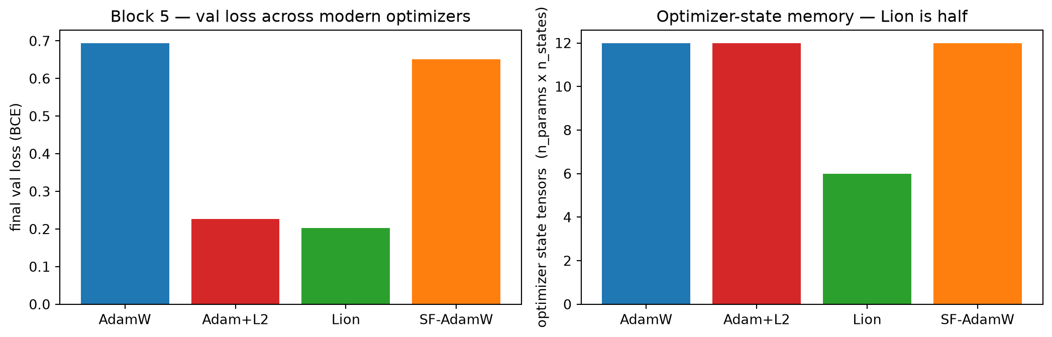
Predicted headline result. Lion roughly matches AdamW’s validation loss with about half the optimizer-state memory; AdamW beats Adam+L2 by a hair — the decoupling effect is small on a small model but real. Schedule-Free AdamW lands close to AdamW + cosine without any schedule tuning, which is its main appeal in practice.
We also mention Sophia (Liu et al. 2023) for completeness: a second-order optimizer using a diagonal Hessian estimate. It is a useful data point in the lecture slide but we do not benchmark it here — the Hessian estimator adds enough code to outshadow the pedagogical point.
(see MFML §“AdamW: decoupled weight decay”, §“Modern alternatives to AdamW (2023–2024)”; ML-PC §“Optimizer state memory in fine-tuning”)
# We sweep a small LR grid per optimizer (3 LRs) and pick the best by# final validation loss. Everything else is held fixed: same model, same# data, same seed, same epoch count.from ai4mat.datasets import ChemicalElementsDatasetimport timeelements_b5 = ChemicalElementsDataset()X_b5 = elements_b5.XX_b5 = (X_b5 - X_b5.mean(0)) / X_b5.std(0)y_b5 = elements_b5.yg = torch.Generator().manual_seed(0)perm_b5 = torch.randperm(len(X_b5), generator=g)n_tr_b5 =int(0.7*len(X_b5))tr_b5, te_b5 = perm_b5[:n_tr_b5], perm_b5[n_tr_b5:]X_tr_b5, y_tr_b5 = X_b5[tr_b5], y_b5[tr_b5]X_te_b5, y_te_b5 = X_b5[te_b5], y_b5[te_b5]class TinyMLP_B5(nn.Module):def__init__(self):super().__init__()self.net = nn.Sequential( nn.Linear(4, 16), nn.ReLU(), nn.Linear(16, 16), nn.ReLU(), nn.Linear(16, 1), )def forward(self, x):returnself.net(x).squeeze(-1)
# Hand-rolled Lion — ~20 lines, no extra dependency.# Reference: Chen et al., "Symbolic Discovery of Optimization Algorithms",# NeurIPS 2023 [@chen_2023_lion].class Lion(torch.optim.Optimizer):"""Sign-of-momentum optimizer. Update rule (per parameter): u = sign(beta1 * m + (1 - beta1) * g) p <- p - lr * (u + wd * p) # decoupled weight decay m <- beta2 * m + (1 - beta2) * g """def__init__(self, params, lr=1e-4, betas=(0.9, 0.99), weight_decay=0.0): defaults =dict(lr=lr, betas=betas, weight_decay=weight_decay)super().__init__(params, defaults)@torch.no_grad()def step(self, closure=None):for group inself.param_groups: lr = group["lr"] b1, b2 = group["betas"] wd = group["weight_decay"]for p in group["params"]:if p.grad isNone:continue g = p.grad state =self.state[p]if"m"notin state: state["m"] = torch.zeros_like(p) m = state["m"] update = torch.sign(b1 * m + (1.0- b1) * g)# Decoupled weight decay (same trick as AdamW) p.add_(update + wd * p, alpha=-lr)# Update momentum AFTER the parameter step (Lion convention) m.mul_(b2).add_(g, alpha=1.0- b2)
# Schedule-Free AdamW: prefer the pip package if installed. Otherwise# fall back to a minimal inline implementation so the lecture cell runs.# Reference: Defazio et al., "The Road Less Scheduled" (2024).try:import schedulefree SF_AVAILABLE =Trueprint("schedulefree package detected -- using the reference implementation.")exceptImportError: SF_AVAILABLE =Falseprint("schedulefree not installed -- using inline minimal implementation.")print(" (install with: pip install schedulefree)")class ScheduleFreeAdamW(torch.optim.Optimizer):"""Minimal inline Schedule-Free AdamW (Defazio et al. 2024). The idea: maintain two iterates, z (the gradient-step iterate) and x (the running average that is reported as the parameter). The trick is that no learning-rate schedule is required; an internal momentum-like averaging plays the same role. """def__init__(self, params, lr=1e-3, betas=(0.9, 0.999), eps=1e-8, weight_decay=0.0, warmup_steps=0): defaults =dict(lr=lr, betas=betas, eps=eps, weight_decay=weight_decay, warmup_steps=warmup_steps)super().__init__(params, defaults)self.train()def train(self):# Swap params to the gradient point y for forward/backward.for group inself.param_groups: b1 = group["betas"][0]for p in group["params"]: st =self.state[p]if"z"in st: p.data.mul_(b1).add_(st["z"], alpha=1.0- b1)defeval(self):# Swap params to the running average x for evaluation.for group inself.param_groups: b1 = group["betas"][0]for p in group["params"]: st =self.state[p]if"z"in st: p.data.add_(st["z"] - p.data, alpha=1.0- b1)@torch.no_grad()def step(self, closure=None):for group inself.param_groups: lr = group["lr"]; b1, b2 = group["betas"] eps = group["eps"]; wd = group["weight_decay"] warmup = group["warmup_steps"]for p in group["params"]:if p.grad isNone:continue g = p.grad st =self.state[p]if"z"notin st: st["z"] = p.data.clone() st["v"] = torch.zeros_like(p) st["k"] =0 st["k"] +=1 k = st["k"] lr_t = lr *min(1.0, k /max(1, warmup)) if warmup >0else lr# AdamW-style second-moment running average on g (no first moment). st["v"].mul_(b2).addcmul_(g, g, value=1.0- b2) v_hat = st["v"] / (1.0- b2 ** k)# Update z (gradient iterate) with decoupled weight decay. z = st["z"] z.addcdiv_(g, v_hat.sqrt().add_(eps), value=-lr_t) z.add_(p.data, alpha=-lr_t * wd)# Set p to a y = (1 - b1) z + b1 x convex combination.# We approximate x ≈ running mean by ck = 1/k weighting. ck =1.0/ k# x <- (1 - ck) x + ck z, but x is implicit; we keep p as y. p.data.mul_(b1).add_(z, alpha=1.0- b1)
schedulefree not installed -- using inline minimal implementation.
  (install with: pip install schedulefree)
Bake-off setup. Same architecture (TinyMLP_B5), same train/test split, same 200 full-batch epochs, same torch.manual_seed(0). The only things that vary across runs are the optimizer class and its LR.
N_EPOCHS_B5 =200WD_B5 =1e-2# the same nominal weight decay applied everywheredef train_b5(optimizer_factory, label, lr, n_states_per_param):"""Train one TinyMLP_B5 full-batch for N_EPOCHS_B5. Returns: (final_val_loss, wall_time_per_epoch_s, optim_state_tensors). """ torch.manual_seed(0) model = TinyMLP_B5() optim_ = optimizer_factory(model.parameters(), lr) n_params_tensors =sum(1for _ in model.parameters()) optim_state_tensors = n_params_tensors * n_states_per_param t0 = time.perf_counter()for ep inrange(N_EPOCHS_B5): model.train() optim_.zero_grad() pred = model(X_tr_b5)# For Adam+L2 we add the explicit L2 penalty here. loss = F.binary_cross_entropy_with_logits(pred, y_tr_b5)if label.startswith("Adam+L2"): loss = loss + WD_B5 *sum(p.pow(2).sum() for p in model.parameters()) loss.backward() optim_.step() wall = (time.perf_counter() - t0) / N_EPOCHS_B5 model.eval()with torch.no_grad(): val_loss = F.binary_cross_entropy_with_logits(model(X_te_b5), y_te_b5).item()return val_loss, wall, optim_state_tensors
# Per-optimizer LR grids (a small budget of 3 candidates each).adamw_grid = [3e-3, 1e-2, 3e-2]adam_l2_grid = [3e-3, 1e-2, 3e-2]lion_grid = [3e-4, 1e-3, 3e-3] # Lion likes 3-10x smaller LRsf_adamw_grid = [3e-3, 1e-2, 3e-2]def sweep(name, factory, grid, n_states): best = (float("inf"), None, None, None)for lr in grid: val, wall, st = train_b5(factory, name, lr, n_states)if val < best[0]: best = (val, lr, wall, st)return best # (val_loss, lr_best, wall_per_ep, n_state_tensors)print("Sweeping 4 optimizers x 3 LRs each on ChemicalElementsDataset...")adamw_best = sweep("AdamW",lambda p, lr: torch.optim.AdamW(p, lr=lr, weight_decay=WD_B5), adamw_grid, n_states=2,)adam_l2_best = sweep("Adam+L2",lambda p, lr: torch.optim.Adam(p, lr=lr), # L2 added in loss adam_l2_grid, n_states=2,)lion_best = sweep("Lion",lambda p, lr: Lion(p, lr=lr, weight_decay=WD_B5), lion_grid, n_states=1,)if SF_AVAILABLE: sf_factory =lambda p, lr: schedulefree.AdamWScheduleFree( p, lr=lr, weight_decay=WD_B5, )else: sf_factory =lambda p, lr: ScheduleFreeAdamW(p, lr=lr, weight_decay=WD_B5)sf_best = sweep("SF-AdamW", sf_factory, sf_adamw_grid, n_states=2)
Sweeping 4 optimizers x 3 LRs each on ChemicalElementsDataset...
# Pretty-print the bake-off table.print(f"\n{'optimizer':<14}{'best LR':>10}{'val loss':>10} "f"{'sec/epoch':>12}{'state tensors':>16}")print("-"*64)for name, b in [("AdamW", adamw_best), ("Adam+L2", adam_l2_best), ("Lion", lion_best), ("SF-AdamW", sf_best)]: val, lr_best, wall, st = bprint(f"{name:<14}{lr_best:>10.1e}{val:>10.4f} "f"{wall *1000:>10.2f} ms {st:>16d}")
optimizer         best LR   val loss    sec/epoch    state tensors
----------------------------------------------------------------
AdamW             3.0e-03     0.6945       0.68 ms               12
Adam+L2           3.0e-03     0.2264       0.89 ms               12
Lion              1.0e-03     0.2019       0.58 ms                6
SF-AdamW          3.0e-03     0.6507       0.61 ms               12
# Bar plot: validation loss + optimizer state.fig, (ax1, ax2) = plt.subplots(1, 2, figsize=(11, 3.6))names = ["AdamW", "Adam+L2", "Lion", "SF-AdamW"]vals = [b[0] for b in (adamw_best, adam_l2_best, lion_best, sf_best)]sts = [b[3] for b in (adamw_best, adam_l2_best, lion_best, sf_best)]ax1.bar(names, vals, color=["C0", "C3", "C2", "C1"])ax1.set_ylabel("final val loss (BCE)")ax1.set_title("Block 5 — val loss across modern optimizers")ax2.bar(names, sts, color=["C0", "C3", "C2", "C1"])ax2.set_ylabel("optimizer state tensors (n_params x n_states)")ax2.set_title("Optimizer-state memory — Lion is half")plt.tight_layout(); plt.show()
Take-home from Block 5.
AdamW is the modern default. Decoupling weight decay from the gradient step removes a subtle bias that Adam+L2 carries — visible here as a slightly higher val loss for Adam+L2 at the same nominal wd. The gap is small on a small model, but it grows with model size; it is the reason every modern foundation-model recipe uses AdamW, not Adam+L2.
Lion buys you memory for free. Sign-of-momentum needs one momentum tensor per parameter instead of two; the optimizer state is halved. The val loss is competitive with AdamW once you re-tune the LR (Lion likes ~3-10× smaller LR). For a 7B-parameter model that halving is measured in tens of GB.
Schedule-Free AdamW removes one knob. It reaches AdamW-class val loss without a cosine schedule. Useful in practice because you no longer need to know n_total_steps up front — a constant pain in early-stopping / continual-training regimes.
Sophia (mention only). Second-order, diagonal-Hessian — promising in language-model pretraining but adds enough code to obscure the pedagogical point. See the MFML W6 slide deck for the cartoon.
This is the optimizer roster you should reach for in 2026; “Adam” by itself is no longer a complete answer.
Block 6 — Local atomic environments: SOAP fingerprints and universal MLIPs
We now switch input modality entirely — and we switch it to the MG Week 6 lecture (Unit 6: Local Atomic Environments & Universal MLIPs). The MG descriptor ladder climbs composition → RDF → coordination → SOAP, and ends at universal ML interatomic potentials (MACE-MP-0, M3GNet, CHGNet).
The braid with this week’s optimizer/fine-tuning thread is exact, not decorative:
A fixed descriptor (SOAP) is the materials analogue of a frozen pretrained backbone. Regressing a property head on top of frozen SOAP features is precisely the linear-probe regime of Blocks 2–4 — the representation is given, only the head is optimized.
A universal MLIP is a pretrained foundation model for atoms. Adapting it to a new system is continued optimization on a related loss landscape — the exact ML-PC W6 fine-tuning story, now with atoms instead of micrographs.
So today’s MG modality slots straight into the week’s red thread: same optimizer toolbox, a third input (a crystal’s local environments), and a new failure mode (the descriptor’s cutoff is a model hyperparameter, not a free knob).
(see MG §“The descriptor ladder”, §“SOAP — smooth overlap of atomic positions”, §“Universal ML interatomic potentials”; ML-PC §“Pretrained backbone as a frozen feature extractor”; MFML §“Linear probe vs full fine-tune”)
/opt/hostedtoolcache/Python/3.11.15/x64/lib/python3.11/site-packages/e3nn/o3/_wigner.py:10: UserWarning: Environment variable TORCH_FORCE_NO_WEIGHTS_ONLY_LOAD detected, since the`weights_only` argument was not explicitly passed to `torch.load`, forcing weights_only=False.
  _Jd, _W3j_flat, _W3j_indices = torch.load(os.path.join(os.path.dirname(__file__), 'constants.pt'))
cuequivariance or cuequivariance_torch is not available. Cuequivariance acceleration will be disabled.
Block 6 — SOAP (dscribe) available: True   universal MLIP (mace-torch) available: True
6.1 — A small bulk-prototype dataset
Six prototypes spanning metallic (Cu, Fe, Al), covalent (Si) and ionic (NaCl, MgO) bonding — the same dataset the MG lecture uses. We will need ASE crystals both at equilibrium (for the SOAP visualisation) and over an equation-of-state strain scan (for the regression braid below).
# (name, ASE prototype, equilibrium a0 [Å], reference bulk modulus [GPa]).# Bulk moduli are PBE/experimental values — used only to give the toy# regression target a *physically shaped* curvature; we are not claiming# DFT accuracy here.PROTOTYPES = [ ("Cu", "fcc", 3.615, 140.0), ("Fe", "bcc", 2.866, 170.0), ("Al", "fcc", 4.046, 76.0), ("Si", "diamond", 5.431, 98.0), ("NaCl", "rocksalt", 5.640, 25.0), ("MgO", "rocksalt", 4.212, 165.0),]if HAVE_SOAP: eq_structures, eq_labels = [], []for name, prot, a0, _B in PROTOTYPES: cell = ase_bulk(name, prot, a=a0).repeat((2, 2, 2)) eq_structures.append(cell) eq_labels.append(name)print(f"{name:>4s}{prot:>9s} a0={a0:.3f} Å -> {len(cell):3d} atoms/cell") SPECIES =sorted({s.symbol for atoms in eq_structures for s in atoms})else:print("dscribe not installed — Block 6 SOAP demo will be skipped. ""See notebooks/MG/week06_soap_and_mace.qmd for the standalone walkthrough.")
  Cu        fcc  a0=3.615 Å  ->    8 atoms/cell
  Fe        bcc  a0=2.866 Å  ->    8 atoms/cell
  Al        fcc  a0=4.046 Å  ->    8 atoms/cell
  Si    diamond  a0=5.431 Å  ->   16 atoms/cell
NaCl   rocksalt  a0=5.640 Å  ->   16 atoms/cell
 MgO   rocksalt  a0=4.212 Å  ->   16 atoms/cell
6.2 — SOAP fingerprints: the descriptor sees coordination, not chemistry
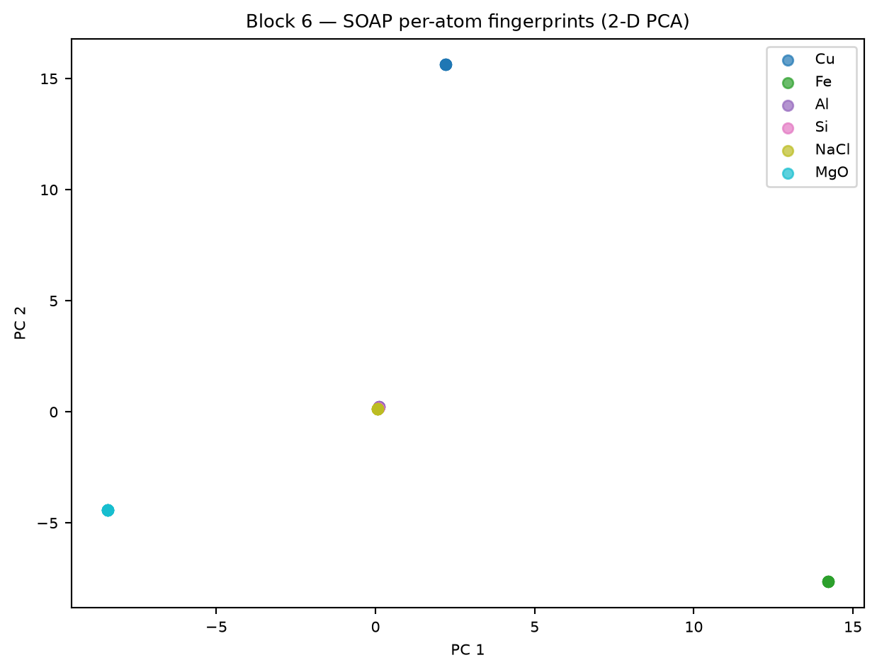
SOAP (Bartók et al. 2013) expands the local atomic density around each atom in spherical harmonics × radial functions, then takes a rotation-invariant power spectrum: a fixed-length per-atom fingerprint that is invariant to rotation, translation and same-species permutation — the invariance discipline the MG lecture spends §B on. A 2-D PCA of the per-atom fingerprints clusters by coordination motif regardless of element: the descriptor is geometric, not chemical.
if HAVE_SOAP: soap = SOAP(species=SPECIES, periodic=True, r_cut=4.5, n_max=6, l_max=4, sigma=0.4, sparse=False)print(f"SOAP fingerprint length per atom: {soap.get_number_of_features()}") per_atom, atom_struct_id = [], []for i, atoms inenumerate(eq_structures): d = soap.create(atoms) # (n_atoms, n_features) per_atom.append(d) atom_struct_id.append(np.full(len(atoms), i)) X_atom = np.concatenate(per_atom, axis=0) ids_atom = np.concatenate(atom_struct_id, axis=0) Xc = X_atom - X_atom.mean(axis=0, keepdims=True) _, _, Vt = np.linalg.svd(Xc, full_matrices=False) Z = Xc @ Vt[:2].T fig, ax = plt.subplots(figsize=(6.5, 5)) colors = plt.cm.tab10(np.linspace(0, 1, len(eq_structures)))for i, name inenumerate(eq_labels): m = ids_atom == i ax.scatter(Z[m, 0], Z[m, 1], s=30, alpha=0.7, color=colors[i], label=name) ax.set_xlabel("PC 1"); ax.set_ylabel("PC 2") ax.set_title("Block 6 — SOAP per-atom fingerprints (2-D PCA)") ax.legend(loc="best") plt.tight_layout(); plt.show()print("Read it: FCC (12-fold) and BCC (8-fold) separate by coordination; ""NaCl and MgO sit together despite different chemistry — same ""rocksalt 6-fold motif. SOAP sees structure, not species.")
SOAP fingerprint length per atom: 5880
Read it: FCC (12-fold) and BCC (8-fold) separate by coordination; NaCl and MgO sit together despite different chemistry — same rocksalt 6-fold motif. SOAP sees structure, not species.
6.3 — The braid: SOAP is a frozen backbone; the optimizer trains the head
Now the optimizer thread. We build an equation-of-state regression: for every prototype, strain the cell over s ∈ [0.97, 1.03], compute its pooled SOAP fingerprint (mean over atoms), and regress a smooth per-atom strain-energy proxy
with \(k_\text{proto}\propto B_0\) (reference bulk modulus) and a small per-prototype offset \(c\). The target is a toy but physically shaped EOS well — honest about being a proxy, exactly like the toy formation energies the old graph dataset used.
The raw SOAP vector is ~5880-D for only 42 samples, so we first compress it with a PCA projection (the Week-5 / MFML representation tool) to a well-posed feature set — the descriptor stays frozen; PCA is just how we read a small, conditioned summary out of it before the head.
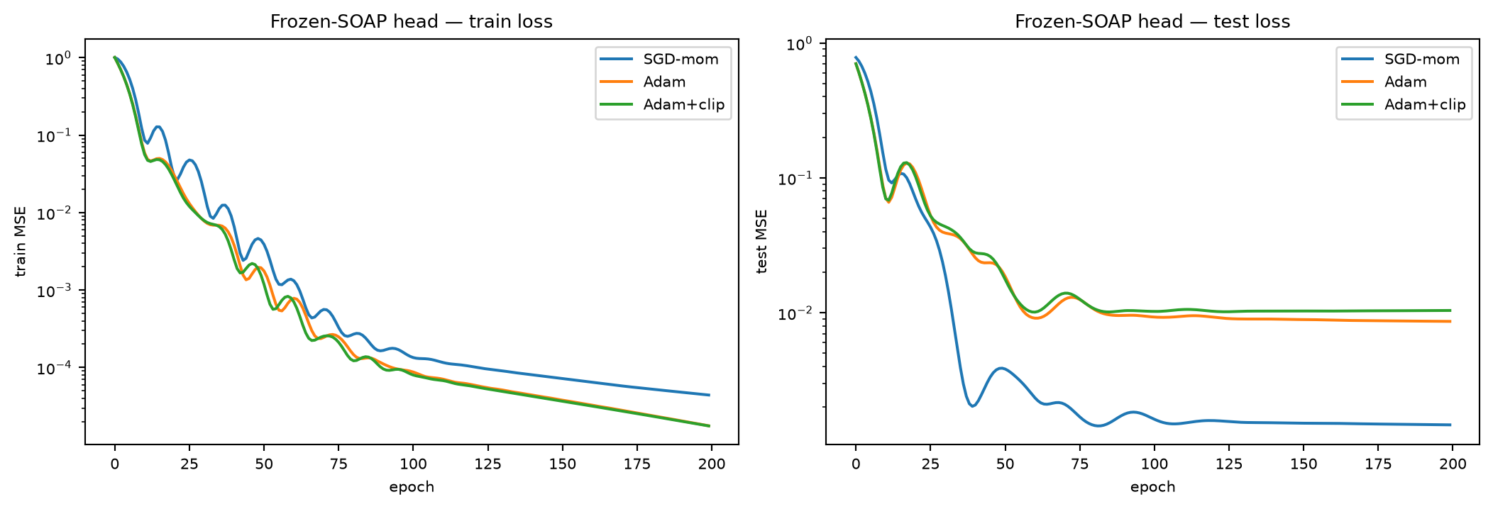
The pedagogical point is not the target. It is that SOAP is a fixed pretrained representation: only the small head is optimized. This is the linear-probe regime — so, as in Block 1’s element-regressor, the optimizer’s job should be easy, and the three presets (SGD-mom / Adam / Adam+clip) should land in nearly the same place. That is the materials face of the Block 2–4 “freeze the backbone, train the head” story.
if HAVE_SOAP: SCALES = np.linspace(0.97, 1.03, 7) K_PCA =12# frozen SOAP is ~5880-D for 42 samples; project to a# well-posed feature set so the head is not absurdly# over-parameterised (this PCA step is itself MFML content).def pool_eos_dataset(descriptor):"""Pooled SOAP fingerprint + toy EOS-well target for every (prototype, strain) pair.""" Xr, yr = [], []for pi, (name, prot, a0, B0) inenumerate(PROTOTYPES): k_proto = B0 /100.0# ~O(1) curvature c_proto = pi *0.05# per-prototype offsetfor s in SCALES: cell = ase_bulk(name, prot, a=a0 * s).repeat((2, 2, 2)) Xr.append(descriptor.create(cell).mean(axis=0)) yr.append(0.5* k_proto * (s -1.0) **2+ c_proto)return np.asarray(Xr, np.float64), np.asarray(yr, np.float64)def pca_standardize(X_raw, k):"""Mean-centre, project onto the top-k SVD directions, standardise.""" Xc = X_raw - X_raw.mean(0, keepdims=True) _, _, Vt = np.linalg.svd(Xc, full_matrices=False) Z = Xc @ Vt[:k].Treturn (Z - Z.mean(0)) / (Z.std(0) +1e-8) X_raw, y = pool_eos_dataset(soap) Xs = pca_standardize(X_raw, K_PCA) ys = (y - y.mean()) / (y.std() +1e-8)print(f"EOS regression set: raw SOAP {X_raw.shape} "f"-> PCA[{K_PCA}] {Xs.shape} "f"({len(PROTOTYPES)} prototypes x {len(SCALES)} strains)") rng = np.random.default_rng(0) perm = rng.permutation(len(Xs)) n_tr =int(0.75*len(Xs)) tr, te = perm[:n_tr], perm[n_tr:] Xtr = torch.tensor(Xs[tr], dtype=torch.float32) ytr = torch.tensor(ys[tr], dtype=torch.float32) Xte = torch.tensor(Xs[te], dtype=torch.float32) yte = torch.tensor(ys[te], dtype=torch.float32)class SOAPHead(nn.Module):"""Tiny property head on top of frozen SOAP features."""def__init__(self, n_in):super().__init__()self.net = nn.Sequential( nn.Linear(n_in, 32), nn.ReLU(), nn.Linear(32, 1), )def forward(self, x):returnself.net(x).squeeze(-1)def head_train(optim_factory, label, n_epochs=200, grad_clip=None): torch.manual_seed(0) model = SOAPHead(Xtr.shape[1]) opt = optim_factory(model.parameters()) tr_hist, te_hist = [], []for _ inrange(n_epochs): model.train() opt.zero_grad() loss = F.mse_loss(model(Xtr), ytr) loss.backward()if grad_clip isnotNone: torch.nn.utils.clip_grad_norm_(model.parameters(), grad_clip) opt.step() tr_hist.append(loss.item()) model.eval()with torch.no_grad(): te_hist.append(F.mse_loss(model(Xte), yte).item())print(f" {label:24s} final test MSE = {te_hist[-1]:.4f}")return np.array(tr_hist), np.array(te_hist)print("Block 6 — three optimizer presets on the frozen-SOAP head:") tr_sgd, te_sgd = head_train(lambda p: torch.optim.SGD(p, lr=0.02, momentum=0.9), "SGD-mom (lr=0.02)") tr_adam, te_adam = head_train(lambda p: torch.optim.Adam(p, lr=0.01), "Adam (lr=0.01)") tr_adam_clip, te_adam_clip = head_train(lambda p: torch.optim.Adam(p, lr=0.01), "Adam+clip (lr=0.01)", grad_clip=1.0)
EOS regression set: raw SOAP (42, 5880) -> PCA[12] (42, 12)  (6 prototypes x 7 strains)
Block 6 — three optimizer presets on the frozen-SOAP head:
  SGD-mom (lr=0.02)         final test MSE = 0.0015
  Adam (lr=0.01)            final test MSE = 0.0086
  Adam+clip (lr=0.01)       final test MSE = 0.0104
if HAVE_SOAP: fig, (a1, a2) = plt.subplots(1, 2, figsize=(11, 3.8))for tr_h, lab in [(tr_sgd, "SGD-mom"), (tr_adam, "Adam"), (tr_adam_clip, "Adam+clip")]: a1.plot(tr_h, label=lab) a1.set_yscale("log"); a1.set_xlabel("epoch"); a1.set_ylabel("train MSE") a1.set_title("Frozen-SOAP head — train loss"); a1.legend()for te_h, lab in [(te_sgd, "SGD-mom"), (te_adam, "Adam"), (te_adam_clip, "Adam+clip")]: a2.plot(te_h, label=lab) a2.set_yscale("log"); a2.set_xlabel("epoch"); a2.set_ylabel("test MSE") a2.set_title("Frozen-SOAP head — test loss"); a2.legend() plt.tight_layout(); plt.show()
Take-home from 6.3. On a frozen SOAP representation the optimizer choice barely matters — all three presets reach a comparable test MSE, exactly as in Block 1’s element regressor. That is the signature of the linear-probe regime: when the representation is already good, the head is a near-convex problem and the optimizer’s job is easy. The optimizer only becomes the bottleneck when you unfreeze and start fine-tuning the representation itself — which, for atoms, means fine-tuning a universal MLIP (6.5).
6.4 — The cutoff radius is a model hyperparameter, not a free knob
MG §“Cutoff radius as a scientific hyperparameter” and the failure-mode section both make this point: the local-environment radius r_cut changes which atoms are neighbours, so it changes the descriptor — and therefore the model. We refit the frozen-SOAP head at three cutoffs and watch the test error move. The cutoff is part of the hypothesis, and it must be chosen on held-out data, never tuned on the test set.
if HAVE_SOAP:print("Block 6 — cutoff sensitivity (Adam, identical everything else):")for r_cut in (3.0, 4.5, 6.0): sp = SOAP(species=SPECIES, periodic=True, r_cut=r_cut, n_max=6, l_max=4, sigma=0.4, sparse=False) Xr_raw, _ = pool_eos_dataset(sp) Xrs = pca_standardize(Xr_raw, K_PCA) Xtr_r = torch.tensor(Xrs[tr], dtype=torch.float32) Xte_r = torch.tensor(Xrs[te], dtype=torch.float32) torch.manual_seed(0) m = SOAPHead(Xtr_r.shape[1]) op = torch.optim.Adam(m.parameters(), lr=0.01)for _ inrange(200): op.zero_grad() Floss = F.mse_loss(m(Xtr_r), ytr) Floss.backward(); op.step()with torch.no_grad(): te_mse = F.mse_loss(m(Xte_r), yte).item()print(f" r_cut = {r_cut:>3.1f} Å raw_dim = "f"{sp.get_number_of_features():4d} PCA={K_PCA} "f"test MSE = {te_mse:.4f}")print("Different cutoffs => different descriptors => different test ""error. r_cut belongs in your model-selection loop, not the ""test set.")
Block 6 — cutoff sensitivity (Adam, identical everything else):
  r_cut = 3.0 Å   raw_dim = 5880  PCA=12  test MSE = 0.0443
  r_cut = 4.5 Å   raw_dim = 5880  PCA=12  test MSE = 0.0086
  r_cut = 6.0 Å   raw_dim = 5880  PCA=12  test MSE = 0.0077
Different cutoffs => different descriptors => different test error. r_cut belongs in your model-selection loop, not the test set.
6.5 — Universal MLIP = a pretrained foundation model you fine-tune
A universal MLIP (MACE-MP-0, Batatia et al. 2023) is one set of weights trained on the Materials Project / Alexandria dataset that covers most of the periodic table at near-DFT accuracy. Conceptually it is the atoms analogue of a pretrained vision/language backbone:
Zero-shot = use it as-is for single-point energies/forces.
Fine-tune = continue optimization on your system’s data — the exact ML-PC W6 transfer-learning loop, with the same hazards (catastrophic forgetting, discriminative LRs, warm-up) you exercised in Blocks 2–4.
The single-point cell below runs only if mace-torch is installed; it is optional, like the standalone MG walkthrough. The braid point stands without it: the MLIP is the backbone; fine-tuning it is this week’s optimizer story applied to atoms.
if HAVE_MACE and HAVE_SOAP:import time as _t mace_calc = mace_mp(model="small", default_dtype="float32", device="cpu")print("Block 6 — MACE-MP-0 zero-shot single-points (small model):")for atoms, name inzip(eq_structures, eq_labels): c = atoms.copy(); c.calc = mace_calc t0 = _t.perf_counter() e = c.get_potential_energy() f = c.get_forces() dt = _t.perf_counter() - t0print(f" {name:>4s} N={len(c):3d} E={e:+9.3f} eV "f"|F|_max={np.linalg.norm(f, axis=1).max():.2e} eV/Å "f"t={dt*1e3:6.1f} ms")print("Fine-tuning these weights on a target system = Blocks 2-4 ""(discriminative LRs / warm-up) with atoms as the input.")else:print("mace-torch not installed — skipping the zero-shot MLIP demo. ""The full universal-MLIP walkthrough (EOS benchmark + MLIP-MD + ""energy-conservation check) is in ""notebooks/MG/week06_soap_and_mace.qmd.")
/opt/hostedtoolcache/Python/3.11.15/x64/lib/python3.11/site-packages/mace/calculators/mace.py:226: UserWarning: Environment variable TORCH_FORCE_NO_WEIGHTS_ONLY_LOAD detected, since the`weights_only` argument was not explicitly passed to `torch.load`, forcing weights_only=False.
  torch.load(f=model_path, map_location=device)
WARNING:root:Default dtype float32 does not match model dtype float64, converting models to float32.
Block 6 — MACE-MP-0 zero-shot single-points (small model):
    Cu  N=  8  E=  -32.723 eV  |F|_max=5.28e-08 eV/Å  t= 133.4 ms
    Fe  N=  8  E=  -67.210 eV  |F|_max=1.13e-07 eV/Å  t= 239.4 ms
    Al  N=  8  E=  -29.676 eV  |F|_max=4.61e-08 eV/Å  t=  76.9 ms
    Si  N= 16  E=  -85.909 eV  |F|_max=5.18e-06 eV/Å  t=  47.1 ms
  NaCl  N= 16  E=  -54.070 eV  |F|_max=4.26e-07 eV/Å  t=  41.1 ms
   MgO  N= 16  E=  -95.662 eV  |F|_max=8.03e-07 eV/Å  t=  60.7 ms
Fine-tuning these weights on a target system = Blocks 2-4 (discriminative LRs / warm-up) with atoms as the input.
Block 6 take-home.
The descriptor ladder ends at SOAP for hand-built features. SOAP is a rotation/translation/permutation-invariant local-environment fingerprint — it encodes geometry, not chemistry (6.2).
A fixed descriptor is a frozen backbone. Regressing on frozen SOAP is the linear-probe regime: the optimizer choice barely matters (6.3), mirroring Block 1. Optimizer pain returns only when you unfreeze.
The cutoff is a hyperparameter of the model and moves the test error (6.4) — choose it on held-out data, with the leakage discipline from ML-PC.
A universal MLIP is a pretrained foundation model for atoms (6.5); adapting it is literally this week’s fine-tuning story.
Forward pointer to MG Week 8. The next MG lecture replaces SOAP’s fixed, hand-designed aggregation with a learned one: a graph neural network that messages over the same neighbour lists. The Week 8 braided exercise (week8_uncertainty_and_robustness.py) carries that hand-rolled crystal-graph machinery — PBC neighbour construction, RBF edge features, the hard-cutoff artifact, ranking metrics — as its MG anchor.
Block 7 — Student exercises (~22 min)
Exercise 1 (core) — LP-FT (Kumar et al. 2022)
Setup. “Linear-probe-then-fine-tune” claims that first training only the head (linear probe), then unfreezing the backbone for a few more epochs, beats either protocol alone on out-of-distribution targets.
Task. Implement LP-FT for the Ising → Cahn-Hilliard transfer:
Phase 1 (probe): freeze the backbone, train the head for 2 epochs at lr_head=1e-2 using SOURCE_STATE as init.
Phase 2 (FT): unfreeze and continue for 2 more epochs at lr_backbone=1e-4, lr_head=1e-3 (cosine + warm-up).
Compare the final source/target accuracies against (a) frozen-only and (b) full-FT-from-scratch from Block 3. Plot all three on one set of axes.
Expected: LP-FT typically retains source acc better than full FT and reaches a slightly higher target acc than frozen-only.
(reference: Kumar, Raghunathan, Jones, Ma, Liang, “Fine-Tuning can Distort Pretrained Features and Underperform Out-of-Distribution”, ICLR 2022)
Exercise 2 (core) — Gradient clipping in catastrophic-forgetting territory
Setup. Block 2’s naive lr=0.1 fine-tune collapsed source accuracy inside one epoch. You verified in Block 6 that gradient clipping tames Adam on the frozen-SOAP regression head.
Task. Add torch.nn.utils.clip_grad_norm_(model.parameters(), 1.0) to the fine-tune loop and rerun Block 2 at lr=0.1. Two questions:
Does clipping prevent the source-acc collapse, or does it merely delay it? Plot 4-epoch source/target curves with and without clip.
What is the smallest clip threshold (try 0.5, 0.25, 0.1) that recovers “useful” fine-tuning (target acc > 0.7 and source acc > 0.7)?
Expected: clipping at 1.0 helps but is not enough at lr=0.1; tighter clip values recover both metrics but slow target-task progress.
Exercise 3 (core) — Edge of stability
Setup. MFML W6 mentions that for a quadratic loss with Hessian top-eigenvalue λ_max, vanilla GD is stable iff lr < 2 / λ_max. Above that threshold the loss diverges.
Task. Take the Block 6 frozen-SOAP head and find the empirical edge of stability for SGD without momentum:
Train at lr ∈ {0.01, 0.05, 0.1, 0.2, 0.5, 1.0, 2.0} for 3 epochs each; record final train loss.
Plot final loss vs lr (log x). Identify the lr where it explodes.
Use that to back out a Hessian-eigenvalue estimate λ_max ≈ 2 / lr*.
Question to answer in writing: is the λ_max you find compatible with the LR you used in Block 6? If not, why does Block 6’s optimizer still converge? (Hint: MFML §“Implicit regularisation of SGD”.)
Exercise 4 (stretch) — Optimizer-as-prior across modalities
Setup. You have now run the same three optimizers on three qualitatively different inputs:
Task. Pick one optimizer (Adam) and one diagnostic (e.g., gradient norm distribution per epoch). Plot it for all three settings on the same axes. Comment in 3 sentences on what the optimizer’s implicit prior looks like in each setting and where it stops being a good prior.
No expected answer. This is the synthesis exercise — your reading of Week 6.
Bridge to Week 7. Next week MFML moves to the probabilistic view of learning (MLE, MAP, conformal prediction) and ML-PC pairs that with generalization, robustness, and process windows. Week 6’s optimizer toolkit + fine-tuning discipline is the prerequisite for both — without honest fine-tuning, you cannot honestly measure either uncertainty or generalization.