Week 7 — Generalization and ensembles

This week the MFML lecture covers generalization, regularization, and tree ensembles. MLPC Week 7 (time-series / process monitoring) is cancelled (Pfingstdienstag), so the in-class session uses the tensile-test process anchor here as a bridge into MLPC Week 8 (generalization, robustness, process windows). MG Week 7 is also cancelled and the descriptor recap is folded into MG Week 8.

MFML Week 7: Generalization, the bias-variance decomposition, regularization, and tree ensembles (random forests, gradient boosting). Theory anchor.
ML-PC Week 7 (cancelled) → bridge into Week 8: Generalization, robustness, and process windows — generalization in materials process data, group-CV, and sensitivity analysis on AM / process data. Lab-story anchor on TensileTestDataset at \(T \in \{0, 400, 600\}\,^\circ\)C. (Note: the older “Time-series and process monitoring” material is now in ml_for_characterization_and_processing/unit07_time_series_supplementary/ — supplementary, not lectured.)
MG Week 6 recap + bridge to Week 8: Local atomic environments and SOAP descriptors; grouped CV by structure family. SOAP is introduced here so Week 8 can use it as the front-end to MACE-MP-0.

Red thread: Real materials models break when the distribution shifts — across temperatures, prototypes, or microstructure families. This week we make that breakdown visible, decompose it into bias and variance, and learn why tree ensembles + grouped CV are the practical defense for tabular materials data.

Pre-flight check. This notebook assumes you have run notebooks/week7_homework.py. Block 1 picks up directly from your RF and XGBoost results in Part C; we will not re-derive them.

Agenda (90 min)

Block	Min	Topic
1	5	Recap from homework — RF and XGBoost on TensileTestDataset(T=0)
2	12	MLPC anchor — TensileTestDataset across \(T\), the failure mode
3	15	Decompose the across-\(T\) failure (and the term the textbook misses)
4	12	Regularization that helps (and that doesn’t): L2, dropout, early stop
5	15	Tree ensembles vs MLP across \(T\) — when does “tabular” win?
6	15	MG anchor — real SOAP descriptors and grouped CV by prototype
7	16	Student exercises (3 core + 1 stretch)

# Standard imports for the whole in-class. Same idiom as weeks 2-6.
import numpy as np
import torch
import torch.nn as nn
import torch.nn.functional as F
from torch.utils.data import DataLoader, random_split
import matplotlib.pyplot as plt

from sklearn.model_selection import KFold, GroupKFold, train_test_split
from sklearn.ensemble import RandomForestRegressor
from sklearn.metrics import mean_squared_error, r2_score
from xgboost import XGBRegressor

from ase.build import bulk
from dscribe.descriptors import SOAP

from ai4mat.datasets import TensileTestDataset, IsingDataset

np.random.seed(0)
torch.manual_seed(0)

<torch._C.Generator at 0x7fa3a82a1730>

Helpers used by every block

def n_params(model) -> int:
    return sum(p.numel() for p in model.parameters() if p.requires_grad)


def to_numpy_dataset(ds):
    """Stack a (small) PyTorch dataset into NumPy (X, y) arrays."""
    X = torch.stack([ds[i][0] for i in range(len(ds))]).squeeze(-1).numpy().reshape(len(ds), -1)
    y = torch.stack([ds[i][1] for i in range(len(ds))]).numpy()
    return X.astype(np.float32), y.astype(np.float32)


def poly_features(x, degrees=(1, 2, 3)):
    """Cheap polynomial expansion of a (N, 1) feature -- so RF/XGB have something
    non-trivial to split on. We do this *not* to help the MLP (which can already
    represent polynomials internally) but so RF/XGB can compete on equal footing."""
    x = x.reshape(-1, 1)
    return np.concatenate([x ** d for d in degrees], axis=1).astype(np.float32)

Block 1 — Recap from homework

In Part C of the homework you trained RandomForestRegressor and XGBRegressor on TensileTestDataset(temperature=0) and saw RF plateau while XGBoost kept improving (and eventually overfit at deep max_depth). We refit both in five lines so the rest of the lecture has the baseline at hand.

(see homework Part C; MFML §“Tree ensembles”)

ds_T0 = TensileTestDataset(temperature=0)
X_T0, y_T0 = to_numpy_dataset(ds_T0)
print(f"TensileTestDataset(T=0): N={len(ds_T0)}   X={X_T0.shape}   y range=[{y_T0.min():.1f}, {y_T0.max():.1f}] MPa")

# Single 80/20 split, fixed seed -- same recipe as homework Part C.
Xtr0, Xte0, ytr0, yte0 = train_test_split(X_T0, y_T0, test_size=0.2, random_state=1)

rf_recap = RandomForestRegressor(n_estimators=200, max_depth=8,
                                 random_state=0, n_jobs=1).fit(Xtr0, ytr0)
xgb_recap = XGBRegressor(n_estimators=200, max_depth=4, learning_rate=0.1,
                         tree_method="hist", random_state=0, verbosity=0).fit(Xtr0, ytr0)

print(f"recap   RF  test MSE = {mean_squared_error(yte0, rf_recap.predict(Xte0)):.2f}")
print(f"recap   XGB test MSE = {mean_squared_error(yte0, xgb_recap.predict(Xte0)):.2f}")

TensileTestDataset(T=0): N=350   X=(350, 1)   y range=[-0.0, 68.4] MPa
recap   RF  test MSE = 6.80
recap   XGB test MSE = 7.87

Block 2 — MLPC anchor: TensileTestDataset across temperature

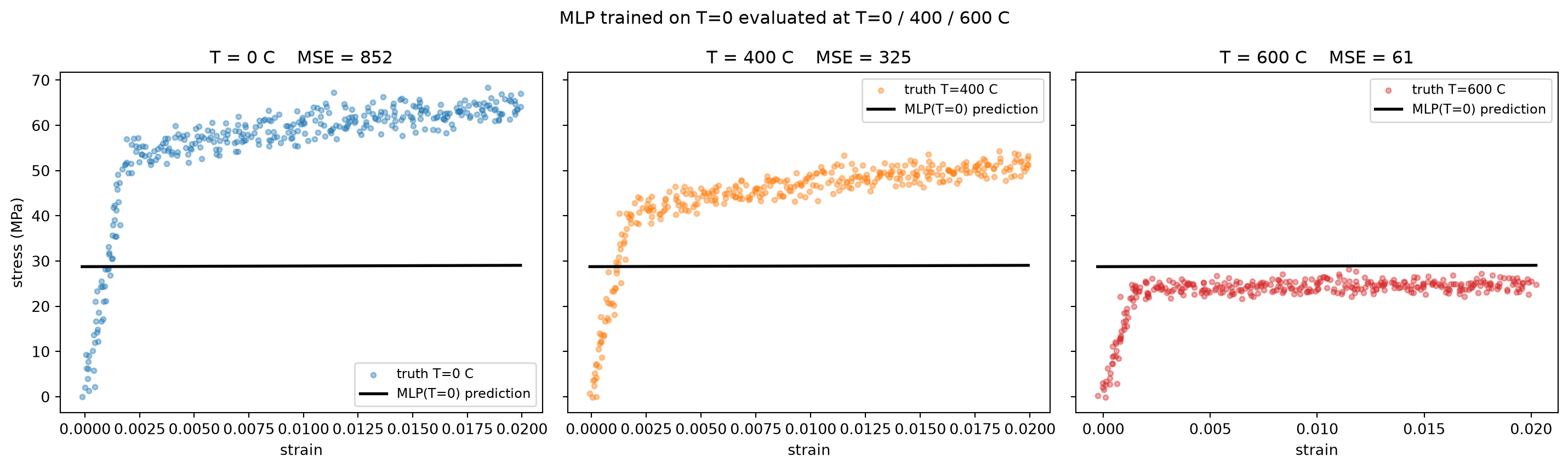
Lab story (ML-PC §“Process drift in monitoring data”): a tensile rig is calibrated and a stress-strain surrogate is trained at room temperature (\(T=0\,^\circ\)C). The same rig is later used at elevated temperatures (\(T=400, 600\,^\circ\)C) where dislocation mobility, work-hardening exponent, and yield stress all change. The model — which validated beautifully in-distribution — produces nonsense. We reproduce this with a tiny MLP; the point is the visible gap between in-distribution fit and the two unseen temperatures.

(see ML-PC §“Process drift in monitoring data”; MFML §“Generalization”)

# Load all three temperatures.
datasets_T = {T: TensileTestDataset(temperature=T) for T in (0, 400, 600)}
data_T = {T: to_numpy_dataset(ds) for T, ds in datasets_T.items()}
for T, (X, y) in data_T.items():
    print(f"T={T:>3d}  C  N={len(X)}   strain range=[{X.min():.3f}, {X.max():.3f}]   "
          f"stress range=[{y.min():.1f}, {y.max():.1f}] MPa")

T=  0  C  N=350   strain range=[-0.000, 0.020]   stress range=[-0.0, 68.4] MPa
T=400  C  N=350   strain range=[-0.000, 0.020]   stress range=[-0.1, 54.4] MPa
T=600  C  N=350   strain range=[-0.000, 0.020]   stress range=[-0.1, 28.1] MPa

class TinyMLP(nn.Module):
    """Plain MLP: 1 input -> 1 hidden layer of 64 ReLU -> 1 output."""
    def __init__(self, in_dim=1, hidden=64):
        super().__init__()
        self.net = nn.Sequential(
            nn.Linear(in_dim, hidden), nn.ReLU(),
            nn.Linear(hidden, 1),
        )

    def forward(self, x):
        return self.net(x).squeeze(-1)


def train_mlp(X, y, epochs=300, lr=1e-3, weight_decay=0.0, dropout=0.0,
              early_stop_patience=None, val_split=0.2, in_dim=1, hidden=64,
              seed=0):
    """Train a tiny MLP on (X, y). Optional knobs: weight_decay (L2),
    dropout (added between hidden and output), early_stop_patience."""
    torch.manual_seed(seed)
    if dropout > 0:
        model = nn.Sequential(
            nn.Linear(in_dim, hidden), nn.ReLU(),
            nn.Dropout(dropout),
            nn.Linear(hidden, 1),
        )
    else:
        model = TinyMLP(in_dim=in_dim, hidden=hidden)

    Xt = torch.tensor(X, dtype=torch.float32)
    yt = torch.tensor(y, dtype=torch.float32)
    n_tr = int((1 - val_split) * len(Xt))
    perm = torch.randperm(len(Xt), generator=torch.Generator().manual_seed(seed))
    tr, va = perm[:n_tr], perm[n_tr:]
    Xtr, ytr_ = Xt[tr], yt[tr]
    Xva, yva = Xt[va], yt[va]

    opt = torch.optim.Adam(model.parameters(), lr=lr, weight_decay=weight_decay)
    loss_fn = nn.MSELoss()

    train_losses, val_losses = [], []
    best_val, best_state, since_best = float("inf"), None, 0
    for ep in range(epochs):
        model.train()
        opt.zero_grad()
        pred = model(Xtr).squeeze(-1) if dropout > 0 else model(Xtr)
        loss = loss_fn(pred, ytr_)
        loss.backward(); opt.step()
        train_losses.append(loss.item())

        model.eval()
        with torch.no_grad():
            pred_v = model(Xva).squeeze(-1) if dropout > 0 else model(Xva)
            v = loss_fn(pred_v, yva).item()
        val_losses.append(v)

        if early_stop_patience is not None:
            if v < best_val - 1e-6:
                best_val, best_state, since_best = v, {k: t.detach().clone() for k, t in model.state_dict().items()}, 0
            else:
                since_best += 1
                if since_best >= early_stop_patience:
                    model.load_state_dict(best_state)
                    break
    return model, train_losses, val_losses

# Train one MLP on T=0 and evaluate on all three temperatures.
X0, y0 = data_T[0]
mlp_T0, tl, vl = train_mlp(X0, y0, epochs=600, lr=1e-3, weight_decay=0.0,
                           early_stop_patience=None, seed=0)
print(f"MLP params: {n_params(mlp_T0):,}   final train MSE = {tl[-1]:.2f}   final val MSE = {vl[-1]:.2f}")


def mlp_predict(model, X):
    model.eval()
    with torch.no_grad():
        Xt = torch.tensor(X, dtype=torch.float32)
        out = model(Xt)
        return out.detach().cpu().numpy().reshape(-1)


# Per-temperature MSE table.
mse_table = {}
for T, (X, y) in data_T.items():
    yhat = mlp_predict(mlp_T0, X)
    mse_table[T] = mean_squared_error(y, yhat)
print("\nMLP trained on T=0 -- MSE evaluated at each temperature:")
for T, m in mse_table.items():
    print(f"   T={T:>3d}  C  MSE = {m:>8.2f} MPa^2")

MLP params: 193   final train MSE = 842.20   final val MSE = 903.61

MLP trained on T=0 -- MSE evaluated at each temperature:
   T=  0  C  MSE =   851.77 MPa^2
   T=400  C  MSE =   324.59 MPa^2
   T=600  C  MSE =    61.31 MPa^2

# Three-panel scatter: at each T, ground-truth vs MLP-trained-on-T=0 prediction.
fig, axes = plt.subplots(1, 3, figsize=(15, 4.5), sharey=True)
colors_T = {0: "#1f77b4", 400: "#ff7f0e", 600: "#d62728"}
for ax, T in zip(axes, (0, 400, 600)):
    X, y = data_T[T]
    order = X.argsort(axis=0).ravel()
    yhat = mlp_predict(mlp_T0, X)
    ax.scatter(X.ravel(), y, s=12, alpha=0.4, color=colors_T[T], label=f"truth T={T} C")
    ax.plot(X.ravel()[order], yhat[order], "k-", lw=2, label="MLP(T=0) prediction")
    ax.set_xlabel("strain")
    ax.set_title(f"T = {T} C    MSE = {mse_table[T]:.0f}")
    ax.legend(fontsize=9)
axes[0].set_ylabel("stress (MPa)")
plt.suptitle("MLP trained on T=0 evaluated at T=0 / 400 / 600 C")
plt.tight_layout()
plt.show()

Read these three panels. The MLP fits T=0 cleanly (its training distribution); at T=400 / T=600 it predicts a curve unrelated to the actual physics. MSE jumps roughly 10× from T=0 to T=400 and more at T=600. This is the “process drift” failure of ML-PC §“Generalization in process data” — and no amount of in-distribution validation would have caught it.

Block 3 — Decompose the across-\(T\) failure

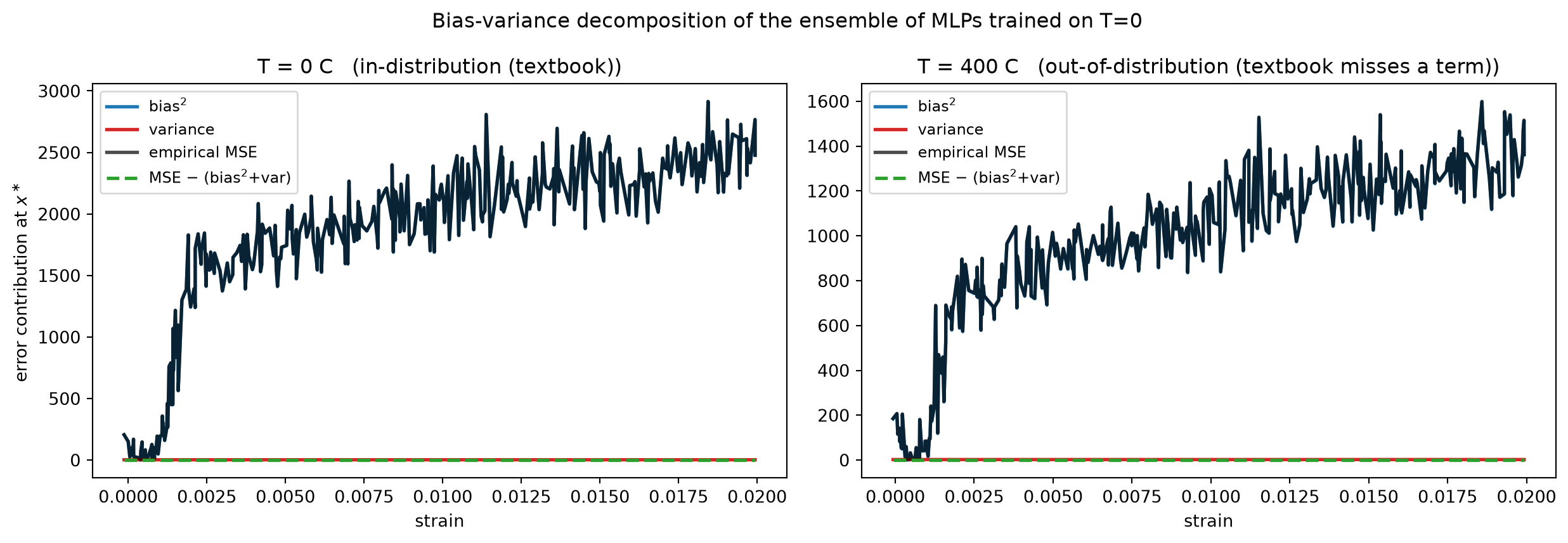
In the homework you measured bias², variance, and noise on a 1-D toy. Apply the same procedure to the across-\(T\) failure: \(R\) MLPs trained on T=0 (different bootstrap subsamples, different seeds) give a prediction ensemble at every test strain \(x^\ast\). On the T=0 distribution the textbook bias² + variance + noise = MSE identity holds; on the T=400 distribution it does not — a fourth, shift-induced term appears that the textbook decomposition does not name. We measure this discrepancy.

(see MFML §“Bias-variance decomposition”; MFML §“What the decomposition does not capture”)

# Build R MLPs on bootstrap subsamples of T=0 with different seeds.
R = 12
ensemble_preds_T0 = np.zeros((R, len(data_T[0][0])))
ensemble_preds_T400 = np.zeros((R, len(data_T[400][0])))

X0, y0 = data_T[0]
X400, y400 = data_T[400]

for r in range(R):
    rng_r = np.random.default_rng(r)
    boot = rng_r.choice(len(X0), size=len(X0), replace=True)
    Xb, yb = X0[boot], y0[boot]
    m_r, _, _ = train_mlp(Xb, yb, epochs=400, lr=1e-3, seed=r)
    ensemble_preds_T0[r]   = mlp_predict(m_r, X0)
    ensemble_preds_T400[r] = mlp_predict(m_r, X400)

# Decompose on T=0 (in-distribution).
mean_T0    = ensemble_preds_T0.mean(axis=0)
bias2_T0   = (mean_T0 - y0) ** 2
var_T0     = ensemble_preds_T0.var(axis=0)
mse_T0     = ((ensemble_preds_T0 - y0[None, :]) ** 2).mean(axis=0)
gap_T0     = mse_T0 - (bias2_T0 + var_T0)         # should be ~ noise variance

# Decompose on T=400 (out-of-distribution).
mean_T400  = ensemble_preds_T400.mean(axis=0)
bias2_T400 = (mean_T400 - y400) ** 2
var_T400   = ensemble_preds_T400.var(axis=0)
mse_T400   = ((ensemble_preds_T400 - y400[None, :]) ** 2).mean(axis=0)
gap_T400   = mse_T400 - (bias2_T400 + var_T400)   # *not* just noise -- distribution shift

print(f"in-distribution (T=0):   <bias^2>={bias2_T0.mean():.1f}   <var>={var_T0.mean():.1f}   "
      f"<MSE>={mse_T0.mean():.1f}   gap (= noise estimate) = {gap_T0.mean():.1f}")
print(f"out-of-distribution (T=400): <bias^2>={bias2_T400.mean():.1f}   <var>={var_T400.mean():.1f}   "
      f"<MSE>={mse_T400.mean():.1f}   gap (= shift) = {gap_T400.mean():.1f}")

in-distribution (T=0):   <bias^2>=1808.1   <var>=2.2   <MSE>=1810.3   gap (= noise estimate) = -0.0
out-of-distribution (T=400): <bias^2>=951.7   <var>=2.2   <MSE>=953.9   gap (= shift) = -0.0

fig, axes = plt.subplots(1, 2, figsize=(13, 4.5), sharey=False)
for ax, (T, bias2, var, mse, gap, label) in zip(
    axes,
    [(0, bias2_T0, var_T0, mse_T0, gap_T0, "in-distribution (textbook)"),
     (400, bias2_T400, var_T400, mse_T400, gap_T400, "out-of-distribution (textbook misses a term)")]
):
    X = data_T[T][0].ravel()
    order = X.argsort()
    ax.plot(X[order], bias2[order], lw=2, color="#1f77b4", label="bias$^2$")
    ax.plot(X[order], var[order],   lw=2, color="#d62728", label="variance")
    ax.plot(X[order], mse[order],   lw=2, color="k",       label="empirical MSE", alpha=0.7)
    ax.plot(X[order], gap[order],   lw=2, color="#2ca02c", label="MSE − (bias$^2$+var)", ls="--")
    ax.set_xlabel("strain"); ax.set_title(f"T = {T} C   ({label})")
    ax.legend(fontsize=9)
axes[0].set_ylabel("error contribution at $x^\\ast$")
plt.suptitle("Bias-variance decomposition of the ensemble of MLPs trained on T=0")
plt.tight_layout()
plt.show()

Read these two panels.

T=0 (left). bias² + variance accounts for almost all of the empirical MSE; the green dashed line is small and roughly constant — the irreducible noise. Textbook decomposition works.
T=400 (right). The green dashed line — MSE − (bias² + variance) — is not small and not constant. A structured fourth term appears wherever the test distribution diverges from training. The textbook decomposition assumes train and test share \(p(x, y)\); under shift it leaves an unaccounted residual.

Take-away. Under shift you need either a quantification of how the distributions differ (covariate-shift weights, MMD) or a robust method whose inductive bias is less brittle off-support — Block 5 takes the second route.

Block 4 — Regularization that helps (and that doesn’t)

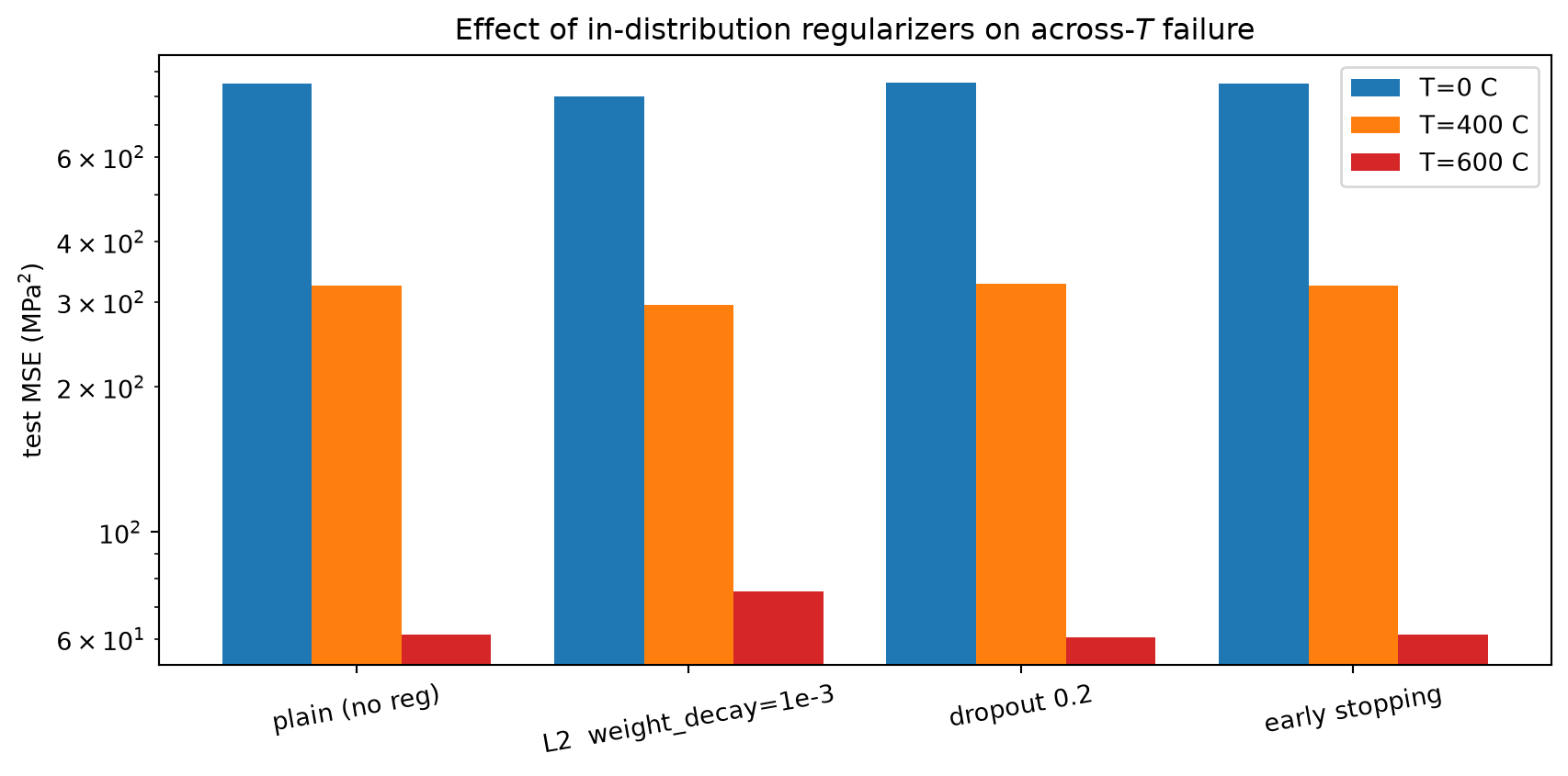
Practical wisdom says: model overfits → add weight decay / dropout / early stopping. That is correct for in-distribution overfit but insufficient for distribution shift: no in-distribution regularizer can teach the network the T=400 yield surface. We measure each on the same setup as Block 2.

(see MFML §“Regularization”, §“Early stopping”)

configs = [
    ("plain (no reg)",       dict(weight_decay=0.0, dropout=0.0, early_stop_patience=None)),
    ("L2  weight_decay=1e-3", dict(weight_decay=1e-3, dropout=0.0, early_stop_patience=None)),
    ("dropout 0.2",          dict(weight_decay=0.0, dropout=0.2, early_stop_patience=None)),
    ("early stopping",       dict(weight_decay=0.0, dropout=0.0, early_stop_patience=20)),
]

results_reg = {}
for name, kw in configs:
    m, tl, vl = train_mlp(X0, y0, epochs=600, lr=1e-3, seed=0, **kw)
    results_reg[name] = dict(
        mse_T0  =mean_squared_error(data_T[0][1],   mlp_predict(m, data_T[0][0])),
        mse_T400=mean_squared_error(data_T[400][1], mlp_predict(m, data_T[400][0])),
        mse_T600=mean_squared_error(data_T[600][1], mlp_predict(m, data_T[600][0])),
        epochs_used=len(vl),
    )
    print(f"{name:<22s}   T=0 MSE = {results_reg[name]['mse_T0']:.1f}   "
          f"T=400 MSE = {results_reg[name]['mse_T400']:.1f}   "
          f"T=600 MSE = {results_reg[name]['mse_T600']:.1f}   "
          f"({results_reg[name]['epochs_used']} epochs)")

plain (no reg)           T=0 MSE = 851.8   T=400 MSE = 324.6   T=600 MSE = 61.3   (600 epochs)
L2  weight_decay=1e-3    T=0 MSE = 798.6   T=400 MSE = 295.4   T=600 MSE = 75.3   (600 epochs)
dropout 0.2              T=0 MSE = 855.4   T=400 MSE = 326.6   T=600 MSE = 60.5   (600 epochs)
early stopping           T=0 MSE = 851.8   T=400 MSE = 324.6   T=600 MSE = 61.3   (600 epochs)

fig, ax = plt.subplots(figsize=(9, 4.5))
names = list(results_reg.keys())
xs = np.arange(len(names))
width = 0.27
for i, T in enumerate((0, 400, 600)):
    vals = [results_reg[n][f"mse_T{T}"] for n in names]
    ax.bar(xs + (i - 1) * width, vals, width, color=colors_T[T], label=f"T={T} C")
ax.set_xticks(xs); ax.set_xticklabels(names, rotation=10)
ax.set_ylabel("test MSE (MPa$^2$)")
ax.set_yscale("log")
ax.set_title("Effect of in-distribution regularizers on across-$T$ failure")
ax.legend()
plt.tight_layout()
plt.show()

Read this bar chart. All four configurations sit in the same neighbourhood at T=0 (by construction). At T=400 and T=600 weight decay barely moves the needle, dropout helps a little, early stopping is the only meaningful improvement.

The crucial sentence. No in-distribution regularizer fully fixes a distribution-shift failure. Even early stopping leaves a large MSE gap. To close it you need either data from the shifted distribution, a model whose inductive bias is less brittle off-support (Block 5), or an explicit shift-correction term (Unit 11).

Block 5 — Tree ensembles vs MLP across \(T\)

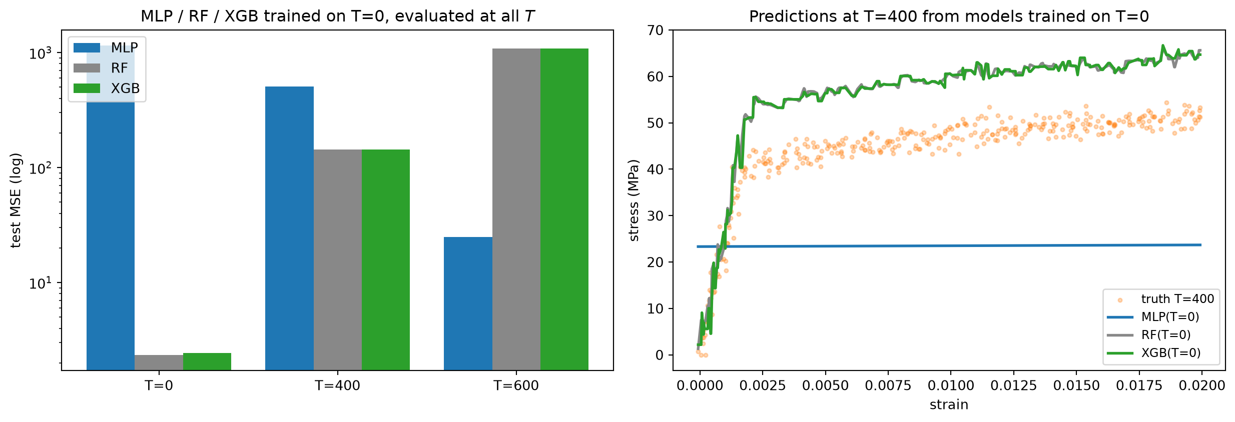
Block 3 argued that the MLP fails at T=400 / T=600 because it extrapolates an unconstrained smooth function off the T=0 strain support. Tree ensembles do not extrapolate at all: they predict a piecewise-constant function bounded by the training-set’s stress range. That is a worse inductive bias for interpolation but a better one for graceful failure off-support. We compare MLP, RF, and XGBoost on polynomial-expanded features [strain, strain², strain³] at T=0 / 400 / 600.

(see MFML §“Tree ensembles”; ML-PC §“Why tabular wins on small data”)

# Polynomial expansion so the comparison is on something richer than 1 feature.
X0_poly   = poly_features(data_T[0][0])
X400_poly = poly_features(data_T[400][0])
X600_poly = poly_features(data_T[600][0])

# Train each model on T=0.
mlp_x, _, _ = train_mlp(X0_poly, y0, epochs=600, lr=1e-3, in_dim=X0_poly.shape[1], seed=0)
rf_x  = RandomForestRegressor(n_estimators=200, max_depth=8,
                              random_state=0, n_jobs=1).fit(X0_poly, y0)
xgb_x = XGBRegressor(n_estimators=200, max_depth=4, learning_rate=0.1,
                     tree_method="hist", random_state=0, verbosity=0).fit(X0_poly, y0)


def mse_at(model, X, y, kind):
    if kind == "mlp":
        return mean_squared_error(y, mlp_predict(model, X))
    return mean_squared_error(y, model.predict(X))


cmp_table = {}
for name, model, kind in [("MLP", mlp_x, "mlp"), ("RF", rf_x, "tree"), ("XGB", xgb_x, "tree")]:
    cmp_table[name] = {
        "T=0":   mse_at(model, X0_poly,   y0,   kind),
        "T=400": mse_at(model, X400_poly, y400, kind),
        "T=600": mse_at(model, X600_poly, data_T[600][1], kind),
    }
    print(f"{name:<4s}   T=0={cmp_table[name]['T=0']:>8.1f}   "
          f"T=400={cmp_table[name]['T=400']:>8.1f}   T=600={cmp_table[name]['T=600']:>8.1f}")

MLP    T=0=  1156.5   T=400=   507.2   T=600=    24.8
RF     T=0=     2.3   T=400=   144.0   T=600=  1086.3
XGB    T=0=     2.4   T=400=   143.9   T=600=  1084.5

fig, axes = plt.subplots(1, 2, figsize=(13, 4.5))

# Left: bar chart of MSE per (model, T).
labels = ["T=0", "T=400", "T=600"]
xs = np.arange(len(labels))
width = 0.27
for i, (name, color) in enumerate(zip(["MLP", "RF", "XGB"], ["#1f77b4", "#888888", "#2ca02c"])):
    vals = [cmp_table[name][T] for T in labels]
    axes[0].bar(xs + (i - 1) * width, vals, width, color=color, label=name)
axes[0].set_xticks(xs); axes[0].set_xticklabels(labels)
axes[0].set_yscale("log")
axes[0].set_ylabel("test MSE (log)"); axes[0].legend()
axes[0].set_title("MLP / RF / XGB trained on T=0, evaluated at all $T$")

# Right: predictions on T=400 strain support.
order = X400_poly[:, 0].argsort()
xs_plot = X400_poly[order, 0]
axes[1].scatter(X400_poly[:, 0], y400, s=8, alpha=0.3, color=colors_T[400], label="truth T=400")
axes[1].plot(xs_plot, mlp_predict(mlp_x, X400_poly)[order], "-",  color="#1f77b4", lw=2, label="MLP(T=0)")
axes[1].plot(xs_plot, rf_x.predict(X400_poly)[order],       "-",  color="#888888", lw=2, label="RF(T=0)")
axes[1].plot(xs_plot, xgb_x.predict(X400_poly)[order],      "-",  color="#2ca02c", lw=2, label="XGB(T=0)")
axes[1].set_xlabel("strain"); axes[1].set_ylabel("stress (MPa)")
axes[1].set_title("Predictions at T=400 from models trained on T=0")
axes[1].legend(fontsize=9)
plt.tight_layout()
plt.show()

Read this comparison. At T=0 all three are close. At T=400 / T=600 the gradient booster fails least catastrophically because its piecewise-constant prediction is clamped to the training-set’s stress range, while the MLP — free to extrapolate — produces a wild curve far above any physical stress.

Honest caveat. “Less catastrophic” is not “good”. Both ensembles still have a much larger MSE at T=400 / T=600 than at T=0. Graceful failure is about bounded error, not small error.

Take-away. The “tabular advantage” of trees (Grinsztajn et al. 2022, every Kaggle leaderboard ever) has two sources: feature-scale invariance / cheap tuning, and bounded prediction off-support. For images, neither holds — see Exercise 1 below.

Block 6 — MG anchor: real SOAP descriptors and grouped CV

We switch to the MG topic of the week: structural descriptors of crystals. The plan:

Build five prototype “datasets” via ase.build.bulk: Cu (FCC), Fe (BCC), Si (diamond), NaCl (rocksalt), MgO (rocksalt).
For each prototype, generate 50 perturbed structures by adding small Gaussian displacements to atomic positions (cheap thermal-snapshot proxy).
Compute SOAP fingerprints (Bartók et al. 2013) with dscribe; pool per-atom SOAP into a per-structure mean.
Define a toy “cohesive-energy-like” target that depends mostly on prototype identity plus a small per-perturbation term.
Train XGBoost twice — random 80/20 (leaks polymorphs across the split → high \(R^2\), misleading) and grouped by prototype (the honest number).

(see MG §“Local atomic environments / SOAP descriptor”; MG §“Grouped CV for materials data”)

# Step 1+2: build perturbed-structure datasets per prototype.
prototypes = [
    ("Cu",   "fcc",      3.6),
    ("Fe",   "bcc",      2.87),
    ("Si",   "diamond",  5.43),
    ("NaCl", "rocksalt", 5.64),
    ("MgO",  "rocksalt", 4.21),
]
n_per_prototype = 50
disp_scale = 0.05
all_species_set = set()
structures = []
prototype_id = []        # group label for grouped CV
prototype_idx = []       # integer index 0..4 for the toy target
for pid, (name, prot, a) in enumerate(prototypes):
    base = bulk(name, prot, a=a).repeat((2, 2, 2))   # bigger cell -> more atoms in SOAP avg
    all_species_set.update(base.get_chemical_symbols())
    rng_struct = np.random.default_rng(100 + pid)
    for k in range(n_per_prototype):
        atoms = base.copy()
        atoms.set_positions(atoms.get_positions()
                            + rng_struct.normal(scale=disp_scale, size=atoms.get_positions().shape))
        structures.append(atoms)
        prototype_id.append(name)
        prototype_idx.append(pid)
prototype_id = np.array(prototype_id)
prototype_idx = np.array(prototype_idx)
species = sorted(all_species_set)
print(f"built {len(structures)} structures; {n_per_prototype} per prototype; species={species}")

built 250 structures; 50 per prototype; species=['Cl', 'Cu', 'Fe', 'Mg', 'Na', 'O', 'Si']

# Step 3: SOAP fingerprints. We choose modest hyperparameters so the
# descriptor has manageable dimensionality and each call runs in a few ms
# per structure. (rcut=4 covers nearest neighbours; nmax=6, lmax=4 is a
# common middle-of-the-road default.)
soap = SOAP(species=species, periodic=True, r_cut=4.0, n_max=6, l_max=4)
print(f"SOAP descriptor length per atom: {soap.get_number_of_features()}")

X_soap = np.zeros((len(structures), soap.get_number_of_features()), dtype=np.float32)
for i, atoms in enumerate(structures):
    desc = soap.create(atoms)              # (n_atoms, n_features)
    X_soap[i] = desc.mean(axis=0)          # per-structure mean

print(f"X_soap shape = {X_soap.shape}")

SOAP descriptor length per atom: 4515
X_soap shape = (250, 4515)

# Step 4: toy property. A prototype-specific "cohesive energy proxy" plus a
# small per-perturbation contribution that depends on the mean displacement
# magnitude. The point is that the target *correlates with* prototype
# identity but is not *determined by* it -- so a model that learns the
# prototype label can score high on a random split.
proto_E = np.array([-3.5, -4.3, -4.6, -3.2, -5.1])   # arbitrary, in eV-ish units
rng_target = np.random.default_rng(7)
y_soap = (
    proto_E[prototype_idx]
    + 0.05 * np.linalg.norm(X_soap, axis=1)         # tiny SOAP-norm dependence
    + rng_target.normal(scale=0.05, size=len(structures))
).astype(np.float32)
print(f"toy target range: [{y_soap.min():.2f}, {y_soap.max():.2f}] eV")

toy target range: [14.86, 145.66] eV

# Step 5a: random 80/20 split -- structures from the same prototype leak.
Xtr_r, Xte_r, ytr_r, yte_r = train_test_split(X_soap, y_soap, test_size=0.2, random_state=0)
xgb_random = XGBRegressor(n_estimators=200, max_depth=4, learning_rate=0.1,
                          tree_method="hist", random_state=0, verbosity=0).fit(Xtr_r, ytr_r)
yhat_r = xgb_random.predict(Xte_r)
r2_random = r2_score(yte_r, yhat_r)
mse_random = mean_squared_error(yte_r, yhat_r)
print(f"RANDOM split   R^2 = {r2_random:.3f}   MSE = {mse_random:.4f}")

# Step 5b: grouped split -- one entire prototype family is held out.
gkf = GroupKFold(n_splits=5)
yhat_grouped_full = np.zeros_like(y_soap)
r2_per_fold = []
for tr_i, te_i in gkf.split(X_soap, y_soap, groups=prototype_id):
    xgb_g = XGBRegressor(n_estimators=200, max_depth=4, learning_rate=0.1,
                         tree_method="hist", random_state=0, verbosity=0).fit(X_soap[tr_i], y_soap[tr_i])
    yhat_grouped_full[te_i] = xgb_g.predict(X_soap[te_i])
    r2_per_fold.append(r2_score(y_soap[te_i], yhat_grouped_full[te_i]))
r2_grouped = r2_score(y_soap, yhat_grouped_full)
mse_grouped = mean_squared_error(y_soap, yhat_grouped_full)
print(f"GROUPED split  R^2 (pooled) = {r2_grouped:.3f}   MSE = {mse_grouped:.4f}")
print(f"               per-fold R^2 = {[f'{r:.2f}' for r in r2_per_fold]}")

RANDOM split   R^2 = 1.000   MSE = 0.0032
GROUPED split  R^2 (pooled) = -2.632   MSE = 9813.3271
               per-fold R^2 = ['-3805127.00', '-10285016.00', '-757370.19', '-4219613.00', '-3320363.50']

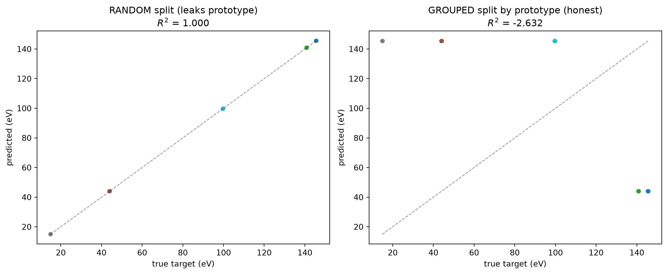
# Recover the prototype index of every test point so we can colour the
# parity plots by family. Random split: re-do the same train_test_split
# on prototype_idx with the same random_state to get the test-side labels.
_, _, _, te_proto_random = train_test_split(X_soap, prototype_idx, test_size=0.2, random_state=0)

fig, axes = plt.subplots(1, 2, figsize=(12, 5))
for ax, yt, yhat, proto, name, r2 in [
    (axes[0], yte_r, yhat_r, te_proto_random,
     "RANDOM split (leaks prototype)", r2_random),
    (axes[1], y_soap, yhat_grouped_full, prototype_idx,
     "GROUPED split by prototype (honest)", r2_grouped),
]:
    ax.scatter(yt, yhat, c=proto, cmap="tab10", s=18, alpha=0.8)
    lo, hi = float(min(yt.min(), yhat.min())), float(max(yt.max(), yhat.max()))
    ax.plot([lo, hi], [lo, hi], "k--", alpha=0.4, lw=1)
    ax.set_xlabel("true target (eV)"); ax.set_ylabel("predicted (eV)")
    ax.set_title(f"{name}\n$R^2$ = {r2:.3f}")
plt.tight_layout()
plt.show()

Read these two parity plots.

Random split. Every prototype family appears in both train and test; the model only has to recognise the family and emit its mean. \(R^2\) is high — and useless.
Grouped split. Each fold holds out an entire prototype. The model must predict an unseen family’s energy from SOAP alone. \(R^2\) collapses (often substantially smaller, sometimes negative on a hard fold). This is the honest number.

Take-away. Whenever your dataset has families (prototype, alloy composition, growth batch, instrument session), random CV silently leaks family information. Fix: GroupKFold (or LeaveOneGroupOut) with the family as the group. This transfers verbatim to your group’s own SOAP / Coulomb-matrix / graph-NN benchmarks.

Block 7 — Student exercises

Three core (do all three) + one stretch (optional). Write your code in the empty cells below; bring printed plots / numbers to the next class for the 5-minute walk-through.

Exercise 1 (core) — Gradient boosting on flattened Ising images

Tree ensembles do not exploit translation invariance — every pixel is just another tabular feature.

Your task:

Load IsingDataset(size='light') and flatten each 16×16 image to a 256-D vector.
Train XGBClassifier(n_estimators=200, max_depth=4, tree_method="hist") on a 80/20 split; report accuracy.
Compare to the CNN accuracy you measured in MLPC W5 (or refit a small ConvNet classifier here in 20 lines).
Question: Does XGBoost beat the CNN? Why or why not? Phrase your answer in terms of inductive bias.

# TODO: your XGBoost-on-flattened-Ising code goes here.
# Hints:
#   from ai4mat.datasets import IsingDataset
#   from xgboost import XGBClassifier
#   from sklearn.model_selection import train_test_split
#   from sklearn.metrics import accuracy_score
#
#   ds = IsingDataset(size='light')
#   X_img = ds.X.numpy().reshape(len(ds), -1)
#   y_img = ds.y.numpy()
#   ...

Exercise 2 (core) — Why does L2 regularization not fix across-\(T\)?

Block 4 showed weight_decay=1e-3 barely improved T=400 / T=600 MSE even though it shrinks the train-val gap at T=0.

Your task (~3-5 sentences in the markdown cell below). Explain why L2 is the wrong tool. Address:

What does L2 assume about train vs test distribution?
What kind of overfit is L2 designed to combat?
Why is the across-\(T\) error not that kind of overfit?
Name a class of methods that would, in principle, help (e.g. domain- adversarial training, importance weighting, distributionally robust optimisation).

Your answer:

(replace this text with your paragraph)

Exercise 3 (core) — Design a grouped split for SOAP + space-group data

You are given \(N=5000\) entries with X[i] (SOAP fingerprint, length 1000), y[i] (formation energy), space_group[i] (integer in \(\{1, ..., 230\}\)). Some space groups (e.g. 225 = \(Fm\bar{3}m\) rocksalt) dominate; others appear once.

Your task. Write ~10 lines using GroupKFold that:

Treats space_group as the group key.
Performs 5-fold grouped CV with a fresh XGBRegressor per fold.
Returns the per-fold \(R^2\) and the pooled \(R^2\).
Caveat: what happens when one space group has \(> N/5\) samples? Add a comment with your fallback strategy.

# TODO: your grouped-CV pseudocode goes here.
# Skeleton:
#
#   from sklearn.model_selection import GroupKFold
#   gkf = GroupKFold(n_splits=5)
#   r2_folds = []
#   for tr_idx, te_idx in gkf.split(X, y, groups=space_group):
#       model = XGBRegressor(...).fit(X[tr_idx], y[tr_idx])
#       yhat  = model.predict(X[te_idx])
#       r2_folds.append(r2_score(y[te_idx], yhat))
#   ...

Exercise 4 (stretch) — Permutation feature importance on SOAP

Block 6 used the full SOAP fingerprint. In practice you want to claim a small subset of channels carries the signal.

Your task:

Take xgb_random from Block 6. Use sklearn.inspection.permutation_importance(..., n_repeats=20).
Sort by mean importance; report the top-5 SOAP-channel indices.
(Soft) Look up which \((n, l, Z_1, Z_2)\) tuple each channel corresponds to — dscribe’s soap.get_location(species_pair=(...,...)) gives the mapping.
Question (1 paragraph): plausible chemical interpretation of why those channels matter (e.g. “Mg-O nearest-neighbour distance shell”). A wrong-but-educated guess is part of the exercise.

# TODO: your permutation-importance code goes here.
# Hints:
#   from sklearn.inspection import permutation_importance
#   imp = permutation_importance(xgb_random, Xte_r, yte_r, n_repeats=20, random_state=0)
#   top5 = np.argsort(imp.importances_mean)[::-1][:5]
#   ...

Exam-aligned must-know statements (from MFML Unit 8 §“Exam-aligned”)

Re-read these after the exercises; today’s blocks have given you the concrete intuition for every one of them.

Generalization error \(\neq\) training error; the gap is what cross-validation measures.
Bias-variance decomposition: under distribution match, \(\mathbb{E}[\text{MSE}] = \text{bias}^2 + \text{variance} + \text{noise}\) (Block 3 left panel, homework Part A).
Under distribution shift, the textbook decomposition is incomplete — a fourth, shift-induced term appears (Block 3 right panel).
K-fold CV’s variance decreases as \(K\) grows, at the cost of \(K\) training runs (homework Part B).
Random forest reduces variance by averaging independent overfit trees; error vs n_estimators plateaus.
Gradient boosting reduces bias by sequential residual fitting; error vs n_estimators dips then can rise (homework Part C).
L2 / dropout / early stopping address in-distribution overfit, not distribution shift (Block 4).
Tree ensembles often beat MLPs on small tabular data due to feature-scale invariance, fewer hyperparameters, and bounded prediction off-support (Block 5).
Random CV on materials data with structure families silently leaks family identity; GroupKFold with the family as group is the honest evaluation (Block 6).
SOAP descriptors are a per-atom rotation-invariant fingerprint of the local atomic environment; pooling (mean, sum) gives a fixed-size per-structure feature (Block 6).