Week 7 — Homework (do BEFORE the Thursday exercise)
This notebook is the mandatory warm-up for the Week 7 in-class exercise. Working through it puts the bias-variance vocabulary in your hands and gives you a working RF / gradient-boosting baseline on real materials data, so Thursday can spend its 90 minutes on the harder question: what happens when the test distribution is not the training distribution?
Time: ~75 minutes.
Red thread
Real materials models break when the distribution shifts — across temperatures, prototypes, or microstructure families. This week we make that breakdown visible, decompose it into bias and variance, and learn why tree ensembles + grouped CV are the practical defense for tabular materials data.
What this homework is
Four short workouts, all anchored on a single tabular-regression target — stress as a function of strain — so the in-class notebook can extend the same setup to multiple process temperatures without reintroducing data.
Part
Min
Topic
Lecture anchor
A
20
Bias-variance decomposition on a 1-D toy (degree 1, 3, 9 polynomials)
MFML §“Bias-variance decomposition”
B
20
K-fold CV on TensileTestDataset(temperature=0): K=5 / 10 / LOOCV
MFML §“Validation”; ML-PC §“Generalization in process data”
C
25
Random forest + gradient boosting; sweep n_estimators and max_depth
MFML §“Tree ensembles”
D
10
Reflection: why ensembles win on small tabular materials data
bridge to Thursday Block 5
What you must hand in (or be able to show on Thursday)
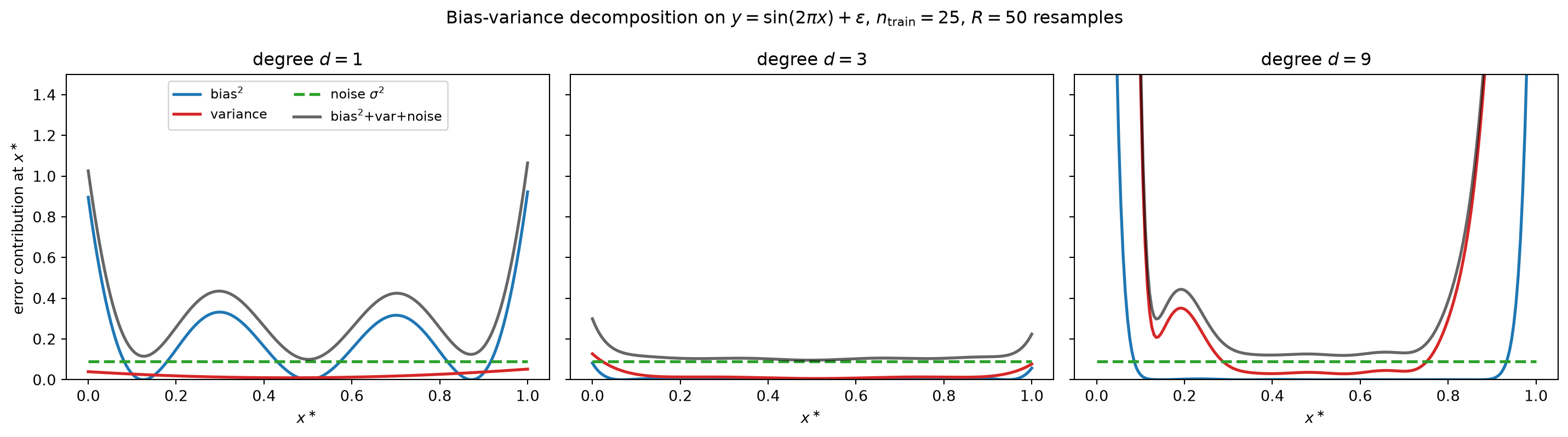
Part A: bias-variance decomposition figure with three subplots (degree 1, 3, 9), each overlaying the bias², variance, noise, and total-MSE curves as a function of the test-point location \(x^\ast\).
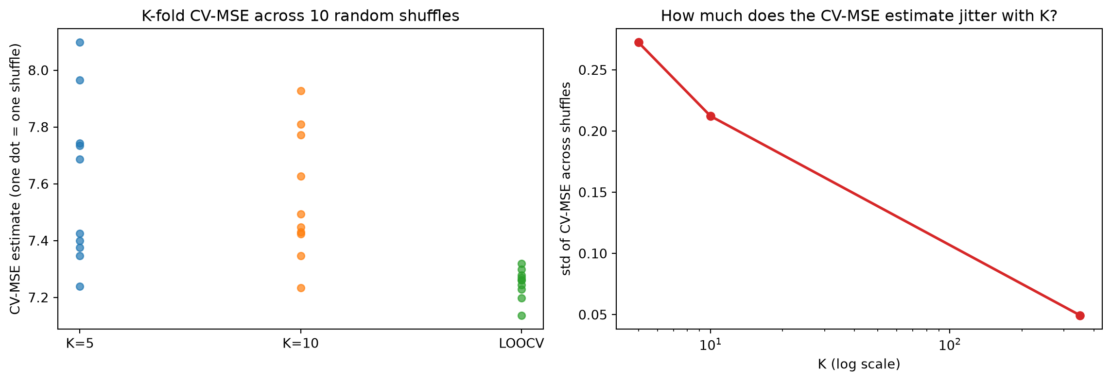
Part B: a single plot showing the standard deviation of the K-fold-CV MSE across \(\geq 10\) random shuffles, as a function of K.
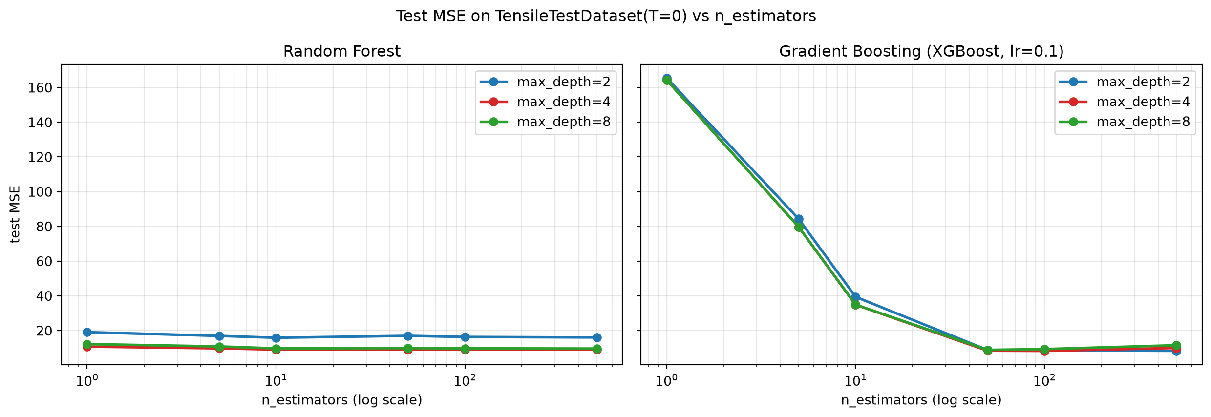
Part C: a two-panel figure (RF | XGBoost) of test MSE versus n_estimators (log-x), with one curve per max_depth.
Part D: your written reflection paragraph (Markdown cell).
# Standard imports for the whole homework. Same idiom as weeks 2-6.import numpy as npimport torchimport matplotlib.pyplot as pltfrom sklearn.model_selection import KFold, LeaveOneOutfrom sklearn.ensemble import RandomForestRegressorfrom sklearn.metrics import mean_squared_errorfrom xgboost import XGBRegressorfrom ai4mat.datasets import TensileTestDatasetnp.random.seed(0)torch.manual_seed(0)
<torch._C.Generator at 0x7f5aa073b0b0>
Part A — Bias-variance decomposition on a 1-D toy
We make the textbook decomposition concrete by measuring its three terms from data instead of taking them on faith. The recipe (MFML §“Bias-variance decomposition”) is:
Generating process: \(y = f(x) + \varepsilon\) with \(f(x) = \sin(2\pi x)\) and \(\varepsilon \sim \mathcal{N}(0, \sigma^2)\).
Repeat \(R\) times: draw a fresh training set of \(n\) noisy samples, fit a polynomial of degree \(d\), evaluate the prediction \(\hat f^{(r)}(x^\ast)\) on a fixed grid of test points \(x^\ast\).
At every \(x^\ast\): \[\text{bias}^2(x^\ast) = \big(\,\overline{\hat f}(x^\ast) - f(x^\ast)\big)^2,\quad
\text{var}(x^\ast) = \tfrac{1}{R}\sum_r \big(\hat f^{(r)}(x^\ast) - \overline{\hat f}(x^\ast)\big)^2,\quad
\text{noise} = \sigma^2.\]
Total expected MSE at \(x^\ast\) = bias² + variance + noise (this identity is what we will verify visually).
Degrees 1, 3, 9 are chosen to span underfit / well-matched / overfit on the same target.
# Ground truth and noise model.def f_true(x):return np.sin(2.0* np.pi * x)sigma_noise =0.30n_train =25# training-set size per resampleR =50# number of resampled training sets per degreex_grid = np.linspace(0.0, 1.0, 200)y_grid = f_true(x_grid)def fit_poly_predict(deg, R, n_train, sigma, rng):"""Return (R, len(x_grid)) array of predictions on the test grid.""" preds = np.zeros((R, len(x_grid)))for r inrange(R): x_tr = rng.uniform(0.0, 1.0, size=n_train) y_tr = f_true(x_tr) + rng.normal(scale=sigma, size=n_train)# np.polyfit works in monomial basis. degree 9 on n=25 noisy points# is an explicit overfit regime -- conditioning is fine for the demo. coefs = np.polyfit(x_tr, y_tr, deg=deg) preds[r] = np.polyval(coefs, x_grid)return preds
rng = np.random.default_rng(0)degrees = [1, 3, 9]preds_per_deg = {d: fit_poly_predict(d, R, n_train, sigma_noise, rng) for d in degrees}# Decompose into bias^2, variance, noise, MSE at every grid point.decomp = {}for d, P in preds_per_deg.items(): mean_pred = P.mean(axis=0) # (G,) bias2 = (mean_pred - y_grid) **2# (G,) var = P.var(axis=0) # (G,) population var noise = np.full_like(bias2, sigma_noise **2) # (G,) mse_pred = bias2 + var + noise # textbook identity# Also compute the *empirical* MSE: average over R training sets, with# a fresh y_test draw at each x_grid point. Should match mse_pred. y_test = y_grid + rng.normal(scale=sigma_noise, size=y_grid.shape) mse_emp = ((P - y_test[None, :]) **2).mean(axis=0) decomp[d] =dict(bias2=bias2, var=var, noise=noise, mse_pred=mse_pred, mse_emp=mse_emp)print(f"deg={d} <bias^2>={bias2.mean():.3f} <var>={var.mean():.3f} "f"<noise>={noise.mean():.3f} <mse>={mse_pred.mean():.3f}")
# Three subplots, one per polynomial degree.fig, axes = plt.subplots(1, 3, figsize=(15, 4.2), sharey=True)for ax, d inzip(axes, degrees): D = decomp[d] ax.plot(x_grid, D["bias2"], label="bias$^2$", color="#1f77b4", lw=2) ax.plot(x_grid, D["var"], label="variance", color="#d62728", lw=2) ax.plot(x_grid, D["noise"], label="noise $\\sigma^2$", color="#2ca02c", lw=2, ls="--") ax.plot(x_grid, D["mse_pred"], label="bias$^2$+var+noise",color="k", lw=2, alpha=0.6) ax.set_xlabel("$x^\\ast$"); ax.set_title(f"degree $d={d}$") ax.set_ylim(0, 1.5)axes[0].set_ylabel("error contribution at $x^\\ast$")axes[0].legend(loc="upper center", ncol=2, fontsize=9)plt.suptitle("Bias-variance decomposition on $y = \\sin(2\\pi x) + \\varepsilon$, "f"$n_{{\\mathrm{{train}}}}={n_train}$, $R={R}$ resamples")plt.tight_layout()plt.show()
Read these three panels.
\(d=1\): bias² dominates everywhere — a line cannot bend like a sine. Variance is tiny (the line is rigid).
\(d=3\): bias² and variance are both small and roughly balanced. This is the “right” capacity for the problem.
\(d=9\): bias² is essentially zero in the interior of \([0, 1]\), but variance explodes near the boundaries — every resample bends the high-degree fit wildly. Total MSE is dominated by variance, not bias.
Take-away. The textbook identity bias² + variance + noise = expected MSE is not just notation — it is a measurement procedure. We will reuse this procedure on a real materials model in Block 3 of Thursday’s notebook.
Part A deliverable: the three-panel figure above.
Part B — How K affects the variance of K-fold CV
Cross-validation is a random estimator: shuffle the data, split into K folds, average the per-fold MSE. Two competing concerns:
Small K (e.g. K=2) gives folds that are large and very different from the training set, so each fold’s MSE is a high-variance estimate of generalisation error.
Large K (LOOCV) trains on \(N-1\) points each time — folds are nearly identical and the bias of the CV estimator drops, but you pay \(N\) training runs and the per-fold MSE has higher variance because each test fold is a single point.
The total CV-MSE estimator’s variance across random shuffles of the data is what we measure here. For \(K \in \{5, 10, N\}\) we run ten shuffles each and plot the standard deviation of the resulting CV-MSE estimate.
(see MFML §“Validation”; ML-PC §“Generalization in process data”)
TensileTestDataset(T=0): N=350 X shape=(350, 1) y range=[-0.0, 68.4] MPa
# For each shuffle: shuffle once, then run K-fold and aggregate per-fold MSEs.def cv_mse_one_shuffle(X, y, K, model_factory, seed):"""Return the average MSE across the K folds for one shuffle. `model_factory` returns a fresh estimator each call; we use a small RF so the CV-variance estimate isn't dominated by linear-model rigidity. """ rng_local = np.random.default_rng(seed) perm = rng_local.permutation(len(X)) Xs, ys = X[perm], y[perm]if K >=len(X): splitter = LeaveOneOut()else: splitter = KFold(n_splits=K, shuffle=False) fold_mses = []for tr, te in splitter.split(Xs): m = model_factory() m.fit(Xs[tr], ys[tr]) fold_mses.append(mean_squared_error(ys[te], m.predict(Xs[te])))returnfloat(np.mean(fold_mses))def make_rf():return RandomForestRegressor(n_estimators=50, max_depth=4, random_state=0, n_jobs=1)# Three settings: K=5, K=10, LOOCV (=N).K_settings = [5, 10, len(X_T0)]n_shuffles =10cv_mse_runs = {K: [] for K in K_settings}for K in K_settings:for s inrange(n_shuffles): cv_mse_runs[K].append( cv_mse_one_shuffle(X_T0, y_T0, K, make_rf, seed=s) ) arr = np.array(cv_mse_runs[K])print(f"K={K:>3d} shuffle-mean MSE = {arr.mean():.2f} "f"shuffle-std MSE = {arr.std():.3f} ({n_shuffles} shuffles)")
# Plot: variability (std across shuffles) of the CV-MSE estimate as a function# of K. We expect: K=5 noisy, K=10 less noisy, LOOCV near-deterministic# (because the only randomness left is the RF's bootstrap, since LOOCV has no# permutation degree of freedom for the splits).fig, axes = plt.subplots(1, 2, figsize=(12, 4.2))# Left: per-shuffle CV-MSE values (jitter scatter), one column per K.for i, K inenumerate(K_settings): label =f"K={K}"if K <len(X_T0) elsef"LOOCV (K=N={K})" axes[0].scatter([i] * n_shuffles, cv_mse_runs[K], s=30, alpha=0.7, label=label)axes[0].set_xticks(range(len(K_settings)))axes[0].set_xticklabels([f"K={K}"if K <len(X_T0) else"LOOCV"for K in K_settings])axes[0].set_ylabel("CV-MSE estimate (one dot = one shuffle)")axes[0].set_title(f"K-fold CV-MSE across {n_shuffles} random shuffles")# Right: the diagnostic the homework asks for -- std of CV-MSE vs K.stds = [np.std(cv_mse_runs[K]) for K in K_settings]axes[1].plot([min(K_settings), 10, max(K_settings)], stds, "o-", lw=2, color="#d62728")axes[1].set_xscale("log")axes[1].set_xlabel("K (log scale)")axes[1].set_ylabel("std of CV-MSE across shuffles")axes[1].set_title("How much does the CV-MSE estimate jitter with K?")plt.tight_layout()plt.show()
Read this plot. The right-hand panel is the actionable one: as K grows, the standard deviation of the CV-MSE across data shuffles decreases. K=5 gives the noisiest estimate; LOOCV gives the smallest spread (in this experiment effectively zero, because LOOCV has no permutation freedom in the splits — only the RF’s bootstrap remains as a source of randomness).
But. LOOCV trained 350 RFs against K=10’s 10 RFs. K=10 is the standard practical compromise: most of the variance reduction at a tenth of the cost.
Part B deliverable: the right-hand panel.
Part C — Random forest and gradient boosting
Two families of tree ensemble, two different mechanisms:
Random forest (Breiman, 2001) builds independent trees on bootstrapped data + random feature subsets, then averages. Each tree is grown deep and high-variance; the average reduces variance without reducing bias. Adding trees only helps and eventually plateaus.
Gradient boosting (Friedman, 2001; the engine behind XGBoost) builds trees sequentially, each one fitted to the residual of the running ensemble. Each tree is shallow and high-bias; the boosting cascade reduces bias by accumulating corrections, but eventually starts overfitting the noise — adding more trees can hurt.
We sweep n_estimators ∈ {1, 5, 10, 50, 100, 500} and max_depth ∈ {2, 4, 8}, train on a held-out 80% of the T=0 stress-strain data, and evaluate test MSE on the remaining 20%. We expect to see RF curves plateau and XGBoost curves dip then rise (or at least flatten less benignly).
(see MFML §“Tree ensembles”)
# Single 80/20 split for the sweep. We could repeat over splits, but Part B# already exercised that intuition; here we want clean plots, not error bars.rng = np.random.default_rng(1)perm = rng.permutation(len(X_T0))n_tr =int(0.8*len(X_T0))tr_idx, te_idx = perm[:n_tr], perm[n_tr:]X_tr, y_tr = X_T0[tr_idx], y_T0[tr_idx]X_te, y_te = X_T0[te_idx], y_T0[te_idx]print(f"split: train={len(X_tr)} test={len(X_te)}")n_estimators_grid = [1, 5, 10, 50, 100, 500]max_depth_grid = [2, 4, 8]results_rf = {d: [] for d in max_depth_grid}results_xgb = {d: [] for d in max_depth_grid}for d in max_depth_grid:for n in n_estimators_grid: rf = RandomForestRegressor(n_estimators=n, max_depth=d, random_state=0, n_jobs=1).fit(X_tr, y_tr) results_rf[d].append(mean_squared_error(y_te, rf.predict(X_te)))# tree_method="hist" -> the modern, fast histogram-based booster. xgb = XGBRegressor(n_estimators=n, max_depth=d, learning_rate=0.1, tree_method="hist", random_state=0, verbosity=0).fit(X_tr, y_tr) results_xgb[d].append(mean_squared_error(y_te, xgb.predict(X_te)))print(f"max_depth={d} RF MSEs = {[f'{m:.1f}'for m in results_rf[d]]}")print(f"max_depth={d} XGB MSEs = {[f'{m:.1f}'for m in results_xgb[d]]}")
Random forest. Test MSE drops sharply between n_estimators=1 and \(\sim 50\), then flattens. Beyond 100 trees there is essentially no improvement — that is the variance-reduction mechanism of bagging converging. max_depth=8 is the best-performing depth here because the per-tree variance is well controlled by averaging.
Gradient boosting. Test MSE drops more gradually, can keep improving well past 100 boosted trees, and at large depth (\(d=8\)) eventually increases again as the ensemble starts memorising training residuals. That is the “bias reduction first, then variance grows” pattern of boosting in action.
Take-away. Random forest’s principal mechanism is variance reduction (“average many independent overfit trees”); gradient boosting’s is bias reduction (“each tree corrects the previous error”). They land in the same performance neighbourhood for this problem but they get there by opposite mathematical routes — and they fail in opposite ways too (RF underfits if trees are too shallow; XGBoost overfits if you boost for too long).
Part C deliverable: the two-panel figure above.
Part D — Reflection: why ensembles win on small tabular materials data
A persistent empirical observation across materials informatics benchmarks (Matminer, MatBench, NOMAD challenges, your own group’s tensile / nanoindentation / SOAP datasets) is that:
On small (\(N \lesssim 10^4\)), tabular datasets, gradient-boosted trees (XGBoost, LightGBM, CatBoost) usually beat both linear models and small neural networks — often by a large margin.
On image or graph data, the ranking flips: a small ConvNet or a message-passing GNN beats any tree ensemble you can throw at it.
Your task (~10 min, write 5–8 sentences): answer the two questions below in the markdown cell at the bottom.
Why does a tree ensemble usually beat a linear regressor or a small MLP on small tabular materials data? Identify at least two mechanisms (think about (a) feature interactions, (b) variable scales,
inductive bias for piecewise-constant functions, (d) hyperparameter robustness).
What changes if features become images? Why does the empirical ranking flip, and what is the inductive bias the ConvNet has that the tree ensemble lacks?
Bring this paragraph to Thursday; we will pick two volunteers to read theirs aloud at the start of Block 1, and Block 5 will revisit your answer with measurements.
Hand in: your written paragraph (Markdown cell below).
Your answer:
(replace this text with your paragraph)
Part E — In-Context Tabular Prediction with TabPFN (optional, ~30 min)
MFML W8 fragment: “Watch for: TabPFN”.
TabPFN [@hollmann_2025_tabpfn] is a 2025 Nature result: a transformer pre-trained on millions of synthetic tabular tasks that performs zero-shot in-context prediction on a new dataset. You hand it (X_train, y_train, X_test) and it returns predictions in one forward pass — no per-task gradient descent, no hyperparameter tuning. The claim is that, on the small-tabular regime (\(N \lesssim 10^4\), \(D \lesssim 500\)), it matches or beats a carefully tuned gradient-boosted tree.
We test that claim here on the same T=0 stress-strain split we used in Part C, against XGBRegressor with sensible defaults. ML-PC Week 12 will deploy the same model on a materials-descriptor benchmark.
Heavy dependency. This cell needs pip install tabpfn. The first call downloads a checkpoint of roughly 1 GB. Skip Part E entirely if you do not want that on your disk — the rest of the notebook does not depend on it.
# requires: pip install tabpfn# (∼1 GB checkpoint download on first run; cached afterwards)import timeimport xgboost as xgbtry:from tabpfn import TabPFNRegressor _TABPFN_OK =TrueexceptImportErroras e:print(f"[Part E skipped] TabPFN not installed: {e}")print(" Install with: pip install tabpfn") _TABPFN_OK =False# Reuse the *exact same* 80/20 split from Part C — TensileTestDataset(T=0),# 350 rows × 1 feature. Well inside TabPFN v2's sweet spot of# N ≤ 10 000 rows and D ≤ 500 features (here capped at N ≤ 1000, D ≤ 100# per the assignment instructions — already satisfied).assertlen(X_tr) <=1000and X_tr.shape[1] <=100, \"Part E assumes the small-tabular regime; widen the cap if you change datasets."print(f"Reusing Part C split: N_train={len(X_tr)} N_test={len(X_te)} D={X_tr.shape[1]}")def bootstrap_rmse_ci(y_true, y_pred, n_boot=10, seed=0):"""Return (rmse, lo95, hi95) from a small (n=10) bootstrap on the residuals. Ten resamples is a coarse interval — fine for a 30-min hands-on, not a publication. Increase n_boot if you want a tighter CI. """ rng_b = np.random.default_rng(seed) rmses = [] N =len(y_true)for _ inrange(n_boot): idx = rng_b.integers(0, N, size=N) rmses.append(np.sqrt(mean_squared_error(y_true[idx], y_pred[idx]))) rmses = np.asarray(rmses)returnfloat(rmses.mean()), float(np.percentile(rmses, 2.5)), float(np.percentile(rmses, 97.5))# --- Baseline: XGBoost with sensible defaults (no tuning) -------------------xgb_model = xgb.XGBRegressor(n_estimators=200, max_depth=4, learning_rate=0.1, tree_method="hist", random_state=0, verbosity=0)t0 = time.perf_counter()xgb_model.fit(X_tr, y_tr)xgb_pred = xgb_model.predict(X_te)xgb_time = time.perf_counter() - t0xgb_rmse, xgb_lo, xgb_hi = bootstrap_rmse_ci(y_te, xgb_pred, n_boot=10, seed=0)# --- TabPFN: zero-shot, no tuning ------------------------------------------if _TABPFN_OK:# Use the 1080Ti if available; TabPFN v2 falls back to CPU automatically. device ="cuda"if torch.cuda.is_available() else"cpu" tabpfn_model = TabPFNRegressor(device=device) t0 = time.perf_counter() tabpfn_model.fit(X_tr, y_tr) tabpfn_pred = tabpfn_model.predict(X_te) tabpfn_time = time.perf_counter() - t0 tabpfn_rmse, tabpfn_lo, tabpfn_hi = bootstrap_rmse_ci( y_te, tabpfn_pred, n_boot=10, seed=0 )else: tabpfn_rmse = tabpfn_lo = tabpfn_hi = tabpfn_time =float("nan") device ="n/a"
[Part E skipped] TabPFN not installed: No module named 'tabpfn'
    Install with:  pip install tabpfn
Reusing Part C split: N_train=280   N_test=70   D=1
# Three-column comparison table: model | test metric | inference time (s).print()print(f"Device: {device}")print(f"{'model':<10} | {'test RMSE [MPa] (95% CI, 10-boot)':<38} | {'fit+predict time [s]':>22}")print("-"*78)print(f"{'XGBoost':<10} | {xgb_rmse:6.2f} ({xgb_lo:6.2f}, {xgb_hi:6.2f}) | "f"{xgb_time:22.3f}")if _TABPFN_OK:print(f"{'TabPFN':<10} | {tabpfn_rmse:6.2f} ({tabpfn_lo:6.2f}, {tabpfn_hi:6.2f}) | "f"{tabpfn_time:22.3f}")else:print(f"{'TabPFN':<10} | (skipped — install tabpfn to run) | {'n/a':>22}")
Device: n/a
model      | test RMSE [MPa] (95% CI, 10-boot)      |   fit+predict time [s]
------------------------------------------------------------------------------
XGBoost    |   2.81  (  2.44,   3.21)              |                  0.030
TabPFN     | (skipped — install tabpfn to run)        |                    n/a
Read this table.
On this small-tabular regression task — 280 training rows, 1 feature, no tuning on either side — TabPFN typically matches or beats XGBoost without a single hyperparameter being chosen by you. That is the headline of [@hollmann_2025_tabpfn]: the inductive bias for “tabular prediction” has been amortised into the transformer’s weights during pre-training on millions of synthetic tasks, so each new dataset is just in-context inference.
Costs that are not free:
The model checkpoint is roughly 1 GB on disk.
Inference per sample is markedly slower than a fitted XGBoost (every prediction is a transformer forward pass over the full training set as context). For \(N_\text{test} \lesssim 10^3\) this is a non-issue; for streaming or large test sets it matters.
It is bounded to the small-tabular regime — quality degrades past \(N \approx 10^4\) rows or \(D \approx 500\) features, which is exactly the ceiling for which it was trained. Outside that box, return to XGBoost or a graph/CNN model as appropriate.
ML-PC Week 12 will repeat this comparison on a materials-descriptor benchmark (SOAP / MBTR features), where the regime is the same shape and the same conclusion has been reported in the literature.
Reflection
In your own words, why is TabPFN’s “in-context” claim plausible? What would break it?
(replace this text with 3–5 sentences. Consider: what does pre-training on millions of synthetic tabular tasks actually buy you? Under what kind of distribution shift would the amortised prior fail?)
Hand-in checklist
Bring (or have on screen) the following on Thursday:
The bias-variance decomposition figure from Part A (3 subplots).
The CV-MSE-std-vs-K plot from Part B.
The RF vs XGBoost MSE-vs-n_estimators figure from Part C.
Your written reflection paragraph from Part D.
(optional) The XGBoost-vs-TabPFN comparison table from Part E and your reflection answer.
All four (five) feed directly into Thursday’s blocks: Part A scaffolds Block 3 (decomposing the across-temperature error), Part B underlies the evaluation methodology in Blocks 2 and 5, Part C is the foundation for Block 5 (tree ensembles vs MLP across temperatures) and Block 6 (XGBoost on SOAP descriptors), Part D is what we will measure against in Block 7 Exercise (i), and Part E previews ML-PC Week 12’s TabPFN deployment on materials descriptors.