Week 8 — Uncertainty and robustness on tensile data
This week braids three lectures:
MFML Week 8 — Probabilistic view of learning. We turn the OLS regression from the homework into an explicit Bayesian model and decompose the predictive variance into aleatoric (irreducible noise) and epistemic (lack of data) parts.
ML-PC Week 8 — Generalisation, robustness, and process windows. We compute input sensitivities and identify the region of the input space where the model is still trustworthy. (The live MLPC exercise slot on 04.06.2026 is cancelled for Fronleichnam, so this block doubles as self-study material for that lecture.)
MG Week 8 — Graph-based crystal representations (Unit 7). After the u06↔︎u07 schedule swap, the MG Week 8 lecture is crystals as graphs: a learned message-passing aggregation replacing the fixed SOAP one. The MG anchor below carries the hand-rolled crystal-graph machinery — PBC neighbour construction, RBF edge features, the hard-cutoff artifact, ranking metrics — and braids it with this week’s optimizer story (a variable-size graph is a rougher loss landscape than the tensile regressors above). (SOAP / universal MLIPs moved to the MG Week 6 lecture and its braided notebook week6_optimization_and_finetuning.py.)
Red thread.Fitting a regression model is making a probabilistic claim: “given \(\mathbf{x}\), my best guess is \(\hat{y}\) with spread \(\hat\sigma\).” Today we make that spread real — first analytically with Bayesian linear regression, then empirically with an ensemble of small neural networks — and we end by drawing the process window: the region of \((\varepsilon, T)\) space where (i) the predicted stress is in spec and (ii) the model’s own self-reported uncertainty is below a threshold. Outside that window, you do not get to use this model.
Pre-flight check. This notebook assumes you have run notebooks/week8_uncertainty_and_robustness_homework.py. Block 1 picks up directly from your MLE = MSE result, Part B’s polynomial sweep, and Part C’s leakage gap; we will not re-derive them.
Agenda (90 min)
Block
Min
Topic
1
6
Recap from homework — MLE = MSE, the U-curve, the leakage gap
rMD17 MLIP energy+force — the correlated-sample trap
9
12
Student exercises (3 core + 1 stretch)
Block 8 is the MG Week 8 anchor: a hand-rolled crystal-graph model (Block 8) and the real crystal-graph machinery (Block 8b — PBC, RBF, ranking metrics). It was moved here from the Week 6 notebook when the MG u06↔︎u07 swap made graph reps the Week 8 lecture.
# Standard imports. Same idiom as weeks 2-6: explicit seeds, no hidden state.import numpy as npimport torchimport torch.nn as nnimport torch.nn.functional as Fimport matplotlib.pyplot as pltfrom sklearn.linear_model import Ridgefrom sklearn.preprocessing import StandardScalerfrom sklearn.metrics import mean_squared_errorfrom ai4mat.datasets import TensileTestDatasetnp.random.seed(0)torch.manual_seed(0)
<torch._C.Generator at 0x7f0954b160d0>
Helpers used by every block
def load_tensile_np(temperature: int):"""Return (strain, stress) at the given temperature as 1-D numpy arrays.""" ds = TensileTestDataset(temperature=temperature)return ds.X.numpy().reshape(-1), ds.y.numpy().reshape(-1)def poly_features(x: np.ndarray, degree: int) -> np.ndarray:"""(N, degree+1) Vandermonde matrix [1, x, x^2, ..., x^d]."""return np.vander(x, degree +1, increasing=True)def standardise_poly(Phi_train: np.ndarray, *Phis: np.ndarray):"""Standardise non-bias columns; share the scaler with held-out matrices.""" scaler = StandardScaler().fit(Phi_train[:, 1:]) out = []for P in (Phi_train, *Phis): out.append(np.hstack([P[:, :1], scaler.transform(P[:, 1:])]))returntuple(out) if Phis else out[0]
Block 1 — Recap from the homework
Three results travel into today’s session:
MLE = MSE. Maximising the Gaussian log-likelihood over coefficients is identical to minimising MSE. The MLE for \(\sigma^2\) is the training MSE. (Part A)
Bias-variance U. Polynomial degree sweep at \(T = 600\) °C: train error keeps falling, test error has a U with the minimum near degree 4-5 for OLS and shifted right for ridge. (Part B)
Leakage gap. A random 80/20 split across \(T \in \{0, 400, 600\}\) looks great; leave-condition-out test RMSE is 5-50× larger. The in-condition U-curve cannot tell you that. (Part C)
Today we make the spread of the prediction the first-class output of the model. We will use the same dataset and the same polynomial basis.
# Load all three temperatures; we will use them in different ways below.data_by_T = {T: load_tensile_np(T) for T in [0, 400, 600]}strain_600, stress_600 = data_by_T[600]print("Block 1 — datasets loaded:")for T in [0, 400, 600]: s, y = data_by_T[T]print(f" T = {T:>3} °C: N = {len(s)}, strain in [{s.min():.3f}, {s.max():.3f}], stress in [{y.min():6.1f}, {y.max():6.1f}] MPa")
Block 1 — datasets loaded:
  T =   0 °C:  N = 350,  strain in [-0.000, 0.020],  stress in [  -0.0,   68.4] MPa
  T = 400 °C:  N = 350,  strain in [-0.000, 0.020],  stress in [  -0.1,   54.4] MPa
  T = 600 °C:  N = 350,  strain in [-0.000, 0.020],  stress in [  -0.1,   28.1] MPa
Block 1b — Leakage-safe cross-validation and the three-set discipline
(ML-PC Week 8 §3 — CV/HPO, and the “test set is sacred” / three-set slides. The live ML-PC slot on 04.06.2026 is cancelled, so this block is the self-study replacement for that material.)
Homework Part C reported a single number per split. One split is one draw of a random variable: it has a variance you never saw. Before we trust any model-selection decision we replace the single split with K-fold cross-validation and report mean ± std across folds.
But K-fold alone is not enough. The single biggest mistake in published materials-ML (the deck’s words) is to K-fold across process conditions: rows from the same specimen / temperature / instrument land in both train and validation, so the score measures interpolation, not generalisation. The fix is a group-aware split that keeps an entire condition out. We contrast:
Protocol
What it estimates
plain 5-fold on \(T = 600\)
error within one condition (optimistic for deployment)
group-K-fold, group = temperature
error on a new, unseen condition (honest)
We then state the three-set discipline explicitly, because every other block in this notebook silently reuses one split:
train — fits the model parameters \(\theta\);
validation — tunes hyperparameters (ridge \(\alpha\), polynomial degree, ensemble size \(M\), the trust threshold in Block 7);
sealed test — touched exactly once, at the very end, to report the number you put in the paper. If you looked at it to make a choice, it is no longer a test set.
sklearn’s KFold / GroupKFold are not imported here on purpose — the fold logic is ten lines and seeing it removes the magic.
def kfold_indices(n: int, k: int, seed: int=0):"""Yield (train_idx, val_idx) for plain shuffled K-fold over n rows.""" rng = np.random.default_rng(seed) perm = rng.permutation(n) folds = np.array_split(perm, k)for i inrange(k): val_idx = folds[i] train_idx = np.concatenate([folds[j] for j inrange(k) if j != i])yield train_idx, val_idxdef group_kfold_indices(groups: np.ndarray):"""Yield (train_idx, val_idx) leaving one whole group out each time. groups is an integer label per row; #folds = #distinct groups. No row from a held-out group ever appears in training — this is the honest 'new condition' estimator. """for g in np.unique(groups): val_idx = np.where(groups == g)[0] train_idx = np.where(groups != g)[0]yield train_idx, val_idx, gdef cv_rmse(strain, stress, splitter, degree=5, alpha=1.0):"""Run a splitter, refit a degree-5 ridge per fold, return per-fold RMSE.""" rmses = []for tr_idx, va_idx in splitter: Phi_tr = poly_features(strain[tr_idx], degree) Phi_va = poly_features(strain[va_idx], degree) Phi_tr_s, Phi_va_s = standardise_poly(Phi_tr, Phi_va) m = Ridge(alpha=alpha, fit_intercept=False).fit(Phi_tr_s, stress[tr_idx]) rmses.append(np.sqrt(mean_squared_error(stress[va_idx], m.predict(Phi_va_s))))return np.array(rmses)# (a) Plain 5-fold *within* T = 600 — the optimistic, in-condition estimate.K =5rmse_kfold = cv_rmse(strain_600, stress_600, kfold_indices(len(strain_600), K, seed=0))# (b) Group-K-fold with group = temperature condition. Each fold holds out# one entire temperature: this is the leave-condition-out estimator,# done K = 3 times so it also gets a mean ± std (homework Part C ran# each leave-T-out exactly once and could not report a spread).strain_grp = np.concatenate([data_by_T[T][0] for T in [0, 400, 600]])stress_grp = np.concatenate([data_by_T[T][1] for T in [0, 400, 600]])group_id = np.concatenate([np.full(len(data_by_T[T][0]), gi)for gi, T inenumerate([0, 400, 600])])rmse_group = cv_rmse( strain_grp, stress_grp, ((tr, va) for tr, va, _g in group_kfold_indices(group_id)),)print("Block 1b — cross-validated test RMSE (degree-5 ridge):")print(f" (a) plain {K}-fold within T = 600 : "f"{rmse_kfold.mean():7.2f} ± {rmse_kfold.std():5.2f} MPa "f"(folds: {np.round(rmse_kfold, 1)})")print(f" (b) group-K-fold, group = T cond. : "f"{rmse_group.mean():7.2f} ± {rmse_group.std():5.2f} MPa "f"(folds: {np.round(rmse_group, 1)})")print(f" honest/optimistic ratio : "f"{rmse_group.mean() / rmse_kfold.mean():.1f}x")print()print(" The single homework-C leave-T=600-out number lives *inside* the")print(" spread of (b); reporting mean ± std is what tells you whether a")print(" model-selection difference is real or just fold noise.")
Block 1b — cross-validated test RMSE (degree-5 ridge):
  (a) plain 5-fold within T = 600 :     3.34 ±  0.26 MPa   (folds: [3.4 3.3 3.2 3.8 3. ])
  (b) group-K-fold, group = T cond. :    19.12 ±  8.64 MPa   (folds: [23.3  7.1 27. ])
  honest/optimistic ratio          :  5.7x

  The single homework-C leave-T=600-out number lives *inside* the
  spread of (b); reporting mean ± std is what tells you whether a
  model-selection difference is real or just fold noise.
Covariate shift made measurable
(ML-PC Week 8 §2 — distribution shift, named and quantified.)
Why does the group split blow up? The deck’s shift taxonomy gives three answers: covariate shift\(p(\mathbf{x})\) moves, label shift\(p(y)\) moves, concept shift\(p(y\mid\mathbf{x})\) moves. Homework Part C showed only the effect (RMSE blow-up). Here we diagnose which shift with a one-line statistic comparison plus a hand-rolled two-sample KS distance — on the strain marginal and on the stress response. The diagnostic matters: covariate shift is fixable by reweighting, concept shift is not.
def ks_distance(a: np.ndarray, b: np.ndarray) ->float:"""Two-sample Kolmogorov–Smirnov statistic sup_x |F_a(x) - F_b(x)|.""" grid = np.sort(np.concatenate([a, b])) Fa = np.searchsorted(np.sort(a), grid, side="right") /len(a) Fb = np.searchsorted(np.sort(b), grid, side="right") /len(b)returnfloat(np.max(np.abs(Fa - Fb)))train_strain = np.concatenate([data_by_T[T][0] for T in [0, 400]])test_strain = data_by_T[600][0]train_stress = np.concatenate([data_by_T[T][1] for T in [0, 400]])test_stress = data_by_T[600][1]ks_x = ks_distance(train_strain, test_strain)ks_y = ks_distance(train_stress, test_stress)print("Block 1b — distribution-shift diagnosis for the leave-T=600-out split:")print(f" strain : train mean={train_strain.mean():.4f} std={train_strain.std():.4f} | "f"test mean={test_strain.mean():.4f} std={test_strain.std():.4f} | "f"KS={ks_x:.3f}")print(f" stress : train mean={train_stress.mean():6.2f} std={train_stress.std():5.2f} | "f"test mean={test_stress.mean():6.2f} std={test_stress.std():5.2f} | "f"KS={ks_y:.3f}")if ks_x <0.1<= ks_y:print(" Diagnosis: the strain marginal is essentially unchanged "f"(KS={ks_x:.3f}) but the")print(" response distribution moves hard (KS_y large). This is NOT ""covariate")print(" shift — it is concept/label shift: same inputs, different ""p(y|x) because")print(" T=600 °C is physically a different material regime. Input ""reweighting")print(" would NOT fix it; only a T-aware model or new data does.")else:print(" Diagnosis: the input marginal itself has moved (covariate ""shift).")print(" Either way this is the same phenomenon as conformal ""exchangeability")print(" failure (homework Part E) and the leakage gap above: a test slice ""that")print(" looked safe but was drawn from a different distribution — one ""failure")print(" at three layers (leakage / shift / broken exchangeability).")
Block 1b — distribution-shift diagnosis for the leave-T=600-out split:
  strain : train mean=0.0094 std=0.0061 | test mean=0.0093 std=0.0061 | KS=0.014
  stress : train mean= 48.73 std=14.02 | test mean= 22.84 std= 4.99 | KS=0.903
  Diagnosis: the strain marginal is essentially unchanged (KS=0.014) but the
  response distribution moves hard (KS_y large). This is NOT covariate
  shift — it is concept/label shift: same inputs, different p(y|x) because
  T=600 °C is physically a different material regime. Input reweighting
  would NOT fix it; only a T-aware model or new data does.
  Either way this is the same phenomenon as conformal exchangeability
  failure (homework Part E) and the leakage gap above: a test slice that
  looked safe but was drawn from a different distribution — one failure
  at three layers (leakage / shift / broken exchangeability).
Three-set discipline, enforced once. Below we build the protocol the rest of the notebook should obey: a train slice fits parameters, a val slice picks the ridge \(\alpha\), and a sealed_test slice is evaluated exactly once at the end. Note the assertion that the three index sets are disjoint — that is the entire “test set is sacred” slide in one line of code.
rng_split = np.random.default_rng(7)perm = rng_split.permutation(len(strain_600))n =len(perm)i_tr, i_va =int(0.6* n), int(0.8* n)train_idx, val_idx, test_idx = perm[:i_tr], perm[i_tr:i_va], perm[i_va:]# Touch-once guarantee: the three sets must not overlap.assertset(train_idx) &set(val_idx) ==set()assert (set(train_idx) |set(val_idx)) &set(test_idx) ==set()# train fits theta, val tunes the hyperparameter alpha (the ONLY thing val# is allowed to influence), test is not looked at during the sweep.best_alpha, best_val =None, np.inffor alpha in [1e-3, 1e-2, 1e-1, 1.0, 10.0]: Phi_tr = poly_features(strain_600[train_idx], 5) Phi_va = poly_features(strain_600[val_idx], 5) Phi_tr_s, Phi_va_s = standardise_poly(Phi_tr, Phi_va) m = Ridge(alpha=alpha, fit_intercept=False).fit(Phi_tr_s, stress_600[train_idx]) v = np.sqrt(mean_squared_error(stress_600[val_idx], m.predict(Phi_va_s)))if v < best_val: best_val, best_alpha = v, alpha# Sealed test: evaluated exactly once, here, with the val-chosen alpha.Phi_tr = poly_features(strain_600[train_idx], 5)Phi_te = poly_features(strain_600[test_idx], 5)Phi_tr_s, Phi_te_s = standardise_poly(Phi_tr, Phi_te)m_final = Ridge(alpha=best_alpha, fit_intercept=False).fit( Phi_tr_s, stress_600[train_idx])sealed_rmse = np.sqrt(mean_squared_error( stress_600[test_idx], m_final.predict(Phi_te_s)))print("Block 1b — three-set protocol on T = 600:")print(f" sizes: train {len(train_idx)} val {len(val_idx)} sealed-test {len(test_idx)}")print(f" val-selected alpha = {best_alpha:g} (val RMSE = {best_val:.2f} MPa)")print(f" SEALED-TEST RMSE = {sealed_rmse:.2f} MPa <-- reported exactly once")print(" If you re-tune anything after reading that last number, it stops")print(" being a test set and the number stops being trustworthy.")
Block 1b — three-set protocol on T = 600:
  sizes: train 210  val 70  sealed-test 70
  val-selected alpha = 0.001  (val RMSE = 2.44 MPa)
  SEALED-TEST RMSE   = 2.12 MPa   <-- reported exactly once
  If you re-tune anything after reading that last number, it stops
  being a test set and the number stops being trustworthy.
Block 2 — Bayesian linear regression
A Bayesian linear regression treats the polynomial coefficients as random variables. With a Gaussian prior \(\mathbf{w} \sim \mathcal{N}(0, \tau^2 \mathbf{I})\) and a Gaussian likelihood \(y \mid \mathbf{x} \sim \mathcal{N}(\boldsymbol\phi(\mathbf{x})^\top \mathbf{w}, \sigma^2)\), the posterior over \(\mathbf{w}\) is also Gaussian: \[
p(\mathbf{w} \mid \mathbf{X}, \mathbf{y})
= \mathcal{N}(\boldsymbol\mu_N, \mathbf{S}_N), \qquad
\mathbf{S}_N^{-1} = \frac{1}{\tau^2}\mathbf{I} + \frac{1}{\sigma^2}\boldsymbol\Phi^\top\boldsymbol\Phi, \qquad
\boldsymbol\mu_N = \frac{1}{\sigma^2}\mathbf{S}_N \boldsymbol\Phi^\top \mathbf{y}.
\] The predictive distribution at a new point \(\mathbf{x}^\star\) is then \[
p(y^\star \mid \mathbf{x}^\star) = \mathcal{N}\!\left(\boldsymbol\phi^\star{}^\top \boldsymbol\mu_N,\ \underbrace{\sigma^2}_\text{aleatoric} + \underbrace{\boldsymbol\phi^\star{}^\top \mathbf{S}_N \boldsymbol\phi^\star}_\text{epistemic}\right).
\] The two terms are exactly the decomposition we will see again in Block 4 from a deep ensemble. The first term is the irreducible noise we cannot remove with more data; the second term shrinks as \(\boldsymbol\Phi^\top\boldsymbol\Phi\) accumulates more samples in the direction of \(\boldsymbol\phi^\star\).
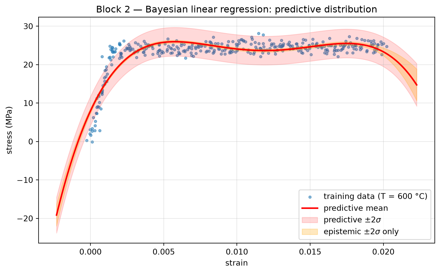
We fit the model on \(T = 600\) °C with a degree-5 polynomial and plot the predictive band over the full strain range.
deg =5strain_grid = np.linspace(strain_600.min() -0.1* (strain_600.max() - strain_600.min()), strain_600.max() +0.1* (strain_600.max() - strain_600.min()),400)Phi_tr = poly_features(strain_600, deg)Phi_grid = poly_features(strain_grid, deg)Phi_tr_s, Phi_grid_s = standardise_poly(Phi_tr, Phi_grid)# Set hyperparameters: sigma^2 from the homework's MLE estimate; tau from# a weak Gaussian prior over standardised coefficients.ols_for_sigma = Ridge(alpha=1e-8, fit_intercept=False).fit(Phi_tr_s, stress_600)sigma2 =float(np.mean((stress_600 - ols_for_sigma.predict(Phi_tr_s)) **2))tau2 =1e3# weak prior; you can sweep it in the exercise# Closed-form posterior over coefficients.D = Phi_tr_s.shape[1]S_N_inv = (1.0/ tau2) * np.eye(D) + (1.0/ sigma2) * (Phi_tr_s.T @ Phi_tr_s)S_N = np.linalg.inv(S_N_inv)mu_N = (1.0/ sigma2) * S_N @ Phi_tr_s.T @ stress_600# Predictive mean and variance on the strain grid.mean_pred = Phi_grid_s @ mu_Nvar_epistemic = np.einsum("ij,jk,ik->i", Phi_grid_s, S_N, Phi_grid_s)var_total = sigma2 + var_epistemicstd_pred = np.sqrt(var_total)print(f"Block 2 — Bayesian linear regression:")print(f" sigma^2 (aleatoric, from training residuals) = {sigma2:.3f}")print(f" tau^2 (prior variance per std coeff) = {tau2:g}")
Block 2 — Bayesian linear regression:
  sigma^2 (aleatoric, from training residuals) = 3.429
  tau^2   (prior variance per std coeff)        = 1000
Notice the two bands. The wide outer band (red) is what the model predicts an individual measurement will look like — it includes the noise floor. The narrow inner band (orange) is the model’s uncertainty about the mean function and shrinks where data is dense, fans out where data is sparse or extrapolated. Bishop Fig. 3.8 is exactly this picture, but on real lab data.
The MAP estimate is the posterior mode. For a Gaussian prior and Gaussian likelihood the posterior is Gaussian, so the MAP coincides with the posterior mean \(\boldsymbol\mu_N\). Working out \(\nabla_\mathbf{w}\log p(\mathbf{w} \mid \mathbf{X}, \mathbf{y}) = 0\) gives \[
\mathbf{w}_\text{MAP} = \big(\boldsymbol\Phi^\top\boldsymbol\Phi + \tfrac{\sigma^2}{\tau^2}\mathbf{I}\big)^{-1} \boldsymbol\Phi^\top \mathbf{y}.
\]This is ridge regression with \(\lambda = \sigma^2 / \tau^2\). Regularisation is not an arbitrary trick to stabilise the fit — it is what falls out of the Bayesian posterior under a Gaussian prior. We verify this numerically.
The two coefficient vectors agree to numerical precision. Whenever you have used Ridge(alpha=...) in this course you have implicitly assumed a Gaussian prior on the standardised coefficients with variance \(\tau^2 = \sigma^2 / \alpha\). Increase \(\alpha\) ↔︎ tighten the prior; decrease \(\alpha\) ↔︎ loosen it. With \(\alpha \to 0\) we recover OLS / MLE; with \(\alpha \to \infty\) we shrink to zero.
Block 4 — Aleatoric vs epistemic via a deep ensemble
The Bayesian polynomial in Block 2 had a closed form because we used a linear model with a Gaussian prior. For a neural network there is no closed form, but we can approximate the same decomposition with a deep ensemble: train \(M\) independently initialised networks on the same data and treat their predictions as samples from an approximate predictive distribution.
Given ensemble outputs \(\hat\mu_m(\mathbf{x})\) for \(m = 1, \dots, M\): \[
\underbrace{\mathrm{Var}_\text{total}(\mathbf{x})}_{\text{predictive variance}}
= \underbrace{\sigma_\text{ale}^2(\mathbf{x})}_{\text{aleatoric, irreducible noise}}
+ \underbrace{\frac{1}{M}\sum_m \big(\hat\mu_m(\mathbf{x}) - \bar\mu(\mathbf{x})\big)^2}_{\text{epistemic, ensemble disagreement}}.
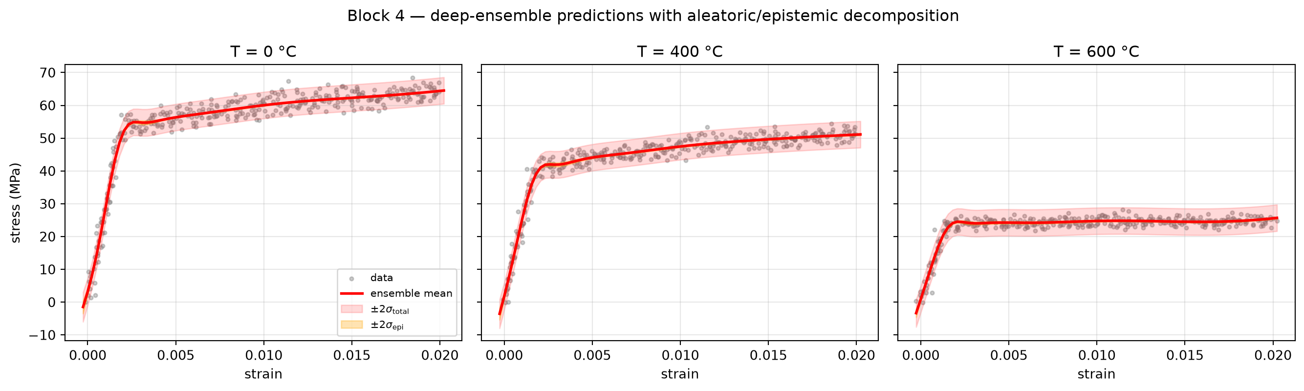
\] We use a small ensemble of MLPs that take the combined data \((\varepsilon, T_\text{norm}) \to \sigma_\text{stress}\), so we can later slice over both axes for the process window.
def make_combined(temps=(0, 400, 600)):"""Return X = (strain, T_norm) and y = stress arrays over multiple temperatures.""" Xs, ys = [], []for T in temps: s, st = load_tensile_np(T) T_norm = np.full_like(s, (T -300.0) /300.0) # roughly [-1, +1] Xs.append(np.stack([s, T_norm], axis=1)) ys.append(st)return np.concatenate(Xs), np.concatenate(ys)X_all, y_all = make_combined()mu_X = X_all.mean(0); sd_X = X_all.std(0) +1e-12mu_y = y_all.mean(); sd_y = y_all.std() +1e-12X_std = (X_all - mu_X) / sd_Xy_std = (y_all - mu_y) / sd_yX_t = torch.tensor(X_std, dtype=torch.float32)y_t = torch.tensor(y_std, dtype=torch.float32)class MLP(nn.Module):def__init__(self, in_dim=2, hidden=64, out_dim=1):super().__init__()self.net = nn.Sequential( nn.Linear(in_dim, hidden), nn.Tanh(), nn.Linear(hidden, hidden), nn.Tanh(), nn.Linear(hidden, out_dim), )def forward(self, x):returnself.net(x).squeeze(-1)def train_one(seed: int, X_t, y_t, n_epochs=400, lr=1e-2, weight_decay=1e-4):"""Train a single MLP from scratch with the given seed; returns the model.""" torch.manual_seed(seed) m = MLP() opt = torch.optim.Adam(m.parameters(), lr=lr, weight_decay=weight_decay)for _ inrange(n_epochs): opt.zero_grad() pred = m(X_t) loss = F.mse_loss(pred, y_t) loss.backward() opt.step()return mM =10print(f"Block 4 — training a deep ensemble (M = {M}) on combined-temperature tensile data ...")ensemble = [train_one(seed=s, X_t=X_t, y_t=y_t) for s inrange(M)]print(f" done.")
Block 4 — training a deep ensemble (M = 10) on combined-temperature tensile data ...
  done.
# Predict on a 2-D grid in (strain, T_norm) for visualisation.strain_grid = np.linspace(X_all[:, 0].min(), X_all[:, 0].max(), 80)T_norm_grid = np.array([(T -300.0) /300.0for T in [0, 400, 600]])SS, TT = np.meshgrid(strain_grid, T_norm_grid)Xq = np.stack([SS.ravel(), TT.ravel()], axis=1)Xq_std = (Xq - mu_X) / sd_XXq_t = torch.tensor(Xq_std, dtype=torch.float32)with torch.no_grad(): preds_std = torch.stack([m(Xq_t) for m in ensemble], dim=0).numpy() # (M, Ngrid)preds = preds_std * sd_y + mu_ymu_bar = preds.mean(axis=0)sigma_epi = preds.std(axis=0) # ensemble disagreementsigma_ale =float(np.sqrt(np.mean( [F.mse_loss(m(X_t), y_t).item() for m in ensemble])) * sd_y) # train residual std, mapped back to MPaprint(f" aleatoric sigma estimate (homoscedastic, MPa): {sigma_ale:.2f}")print(f" epistemic std on grid: min = {sigma_epi.min():.2f}, max = {sigma_epi.max():.2f} MPa")
  aleatoric sigma estimate (homoscedastic, MPa): 2.02
  epistemic std on grid:  min = 0.07, max = 1.00 MPa
# Plot predictions over strain at each of the three temperatures, with# ±2σ_total bands. Aleatoric is the homoscedastic noise floor.fig, axes = plt.subplots(1, 3, figsize=(14, 4.2), sharey=True)for ax, T_norm, T_label inzip(axes, T_norm_grid, [0, 400, 600]): sel = (TT.ravel() == T_norm) s_axis = SS.ravel()[sel] mu = mu_bar[sel] epi = sigma_epi[sel] total = np.sqrt(epi **2+ sigma_ale **2) s_data, st_data = data_by_T[T_label] ax.scatter(s_data, st_data, s=8, alpha=0.4, color="gray", label="data") ax.plot(s_axis, mu, "r-", lw=2, label="ensemble mean") ax.fill_between(s_axis, mu -2* total, mu +2* total, color="red", alpha=0.15, label=r"$\pm 2\sigma_\mathrm{total}$") ax.fill_between(s_axis, mu -2* epi, mu +2* epi, color="orange", alpha=0.3, label=r"$\pm 2\sigma_\mathrm{epi}$") ax.set_title(fr"T = {T_label} °C") ax.set_xlabel("strain") ax.grid(alpha=0.3)axes[0].set_ylabel("stress (MPa)")axes[0].legend(loc="lower right", fontsize=8)fig.suptitle("Block 4 — deep-ensemble predictions with aleatoric/epistemic decomposition")plt.tight_layout()plt.show()
Interpretation:
The orange band is the ensemble’s disagreement at each \((\varepsilon, T)\). It is small wherever many training points support the prediction and grows whenever you move into a region the ensemble has not seen.
The red band adds the irreducible noise floor \(\sigma_\text{ale}\).
The total band is what you would quote to a process engineer as “stress predicted at \(\hat\mu \pm 2\sigma_\text{total}\)”.
Block 5 — Calibration: does \(\hat\sigma\) match reality?
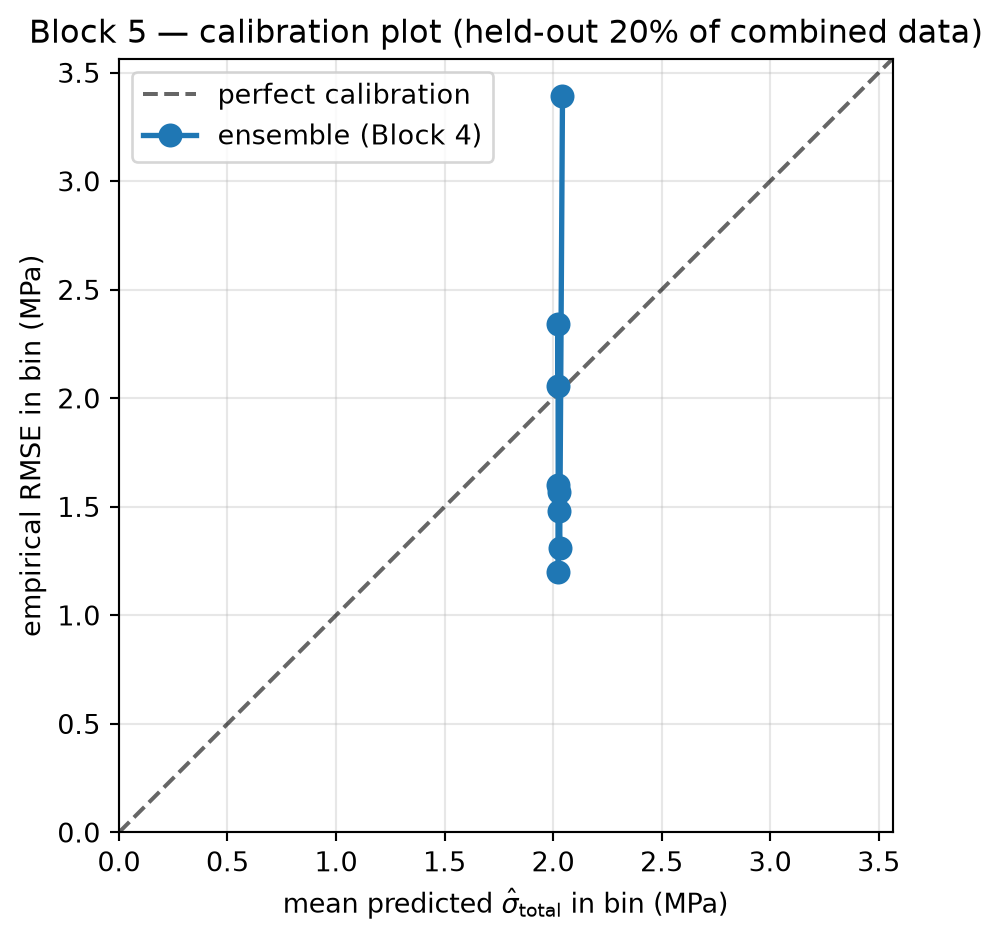
A model that predicts mean and variance is calibrated if the empirical error in each \(\hat\sigma\) bin matches that bin’s \(\hat\sigma\). We evaluate this on a held-out 20% slice of the combined data.
rng = np.random.default_rng(2)N =len(X_all)idx = rng.permutation(N)ntr =int(0.8* N)te_idx = idx[ntr:]X_te = X_t[te_idx]y_te = y_all[te_idx]with torch.no_grad(): preds_te_std = torch.stack([m(X_te) for m in ensemble], dim=0).numpy()preds_te = preds_te_std * sd_y + mu_ymu_te = preds_te.mean(axis=0)sigma_epi_te = preds_te.std(axis=0)sigma_total_te = np.sqrt(sigma_epi_te **2+ sigma_ale **2)abs_err = np.abs(mu_te - y_te)# Bin test points into 8 quantile bins of predicted sigma_total.n_bins =8order = np.argsort(sigma_total_te)chunks = np.array_split(order, n_bins)mean_pred_sigma = np.array([sigma_total_te[c].mean() for c in chunks])mean_emp_rmse = np.array([np.sqrt(np.mean((mu_te[c] - y_te[c]) **2)) for c in chunks])print("Block 5 — calibration table:")print(f" {'bin':>4}{'mean pred sigma':>16}{'empirical RMSE':>16}")for i, (ps, er) inenumerate(zip(mean_pred_sigma, mean_emp_rmse)):print(f" {i+1:>4}{ps:>16.3f}{er:>16.3f}")
fig, ax = plt.subplots(figsize=(6, 5))m_lim =max(mean_pred_sigma.max(), mean_emp_rmse.max()) *1.05ax.plot([0, m_lim], [0, m_lim], "k--", alpha=0.6, label="perfect calibration")ax.plot(mean_pred_sigma, mean_emp_rmse, "o-", lw=2, ms=8, label="ensemble (Block 4)")ax.set_xlabel(r"mean predicted $\hat\sigma_\mathrm{total}$ in bin (MPa)")ax.set_ylabel("empirical RMSE in bin (MPa)")ax.set_title("Block 5 — calibration plot (held-out 20% of combined data)")ax.set_xlim(0, m_lim); ax.set_ylim(0, m_lim)ax.set_aspect("equal")ax.grid(alpha=0.3); ax.legend()plt.tight_layout(); plt.show()
The diagonal is perfect calibration: when you say \(\hat\sigma = 50\) MPa the average error in that bin should be 50 MPa. Above the line means under-confident (you said 50, you got 80 — your model is more wrong than it admits). Below the line means over-confident. With a 10-member ensemble and homoscedastic aleatoric, expect to be under-confident in low-data regions and over-confident on the noise floor. Block 8 Exercise 3 asks you to fix the binning and revisit this.
Block 6 — Sensitivity analysis on \((\varepsilon, T)\)
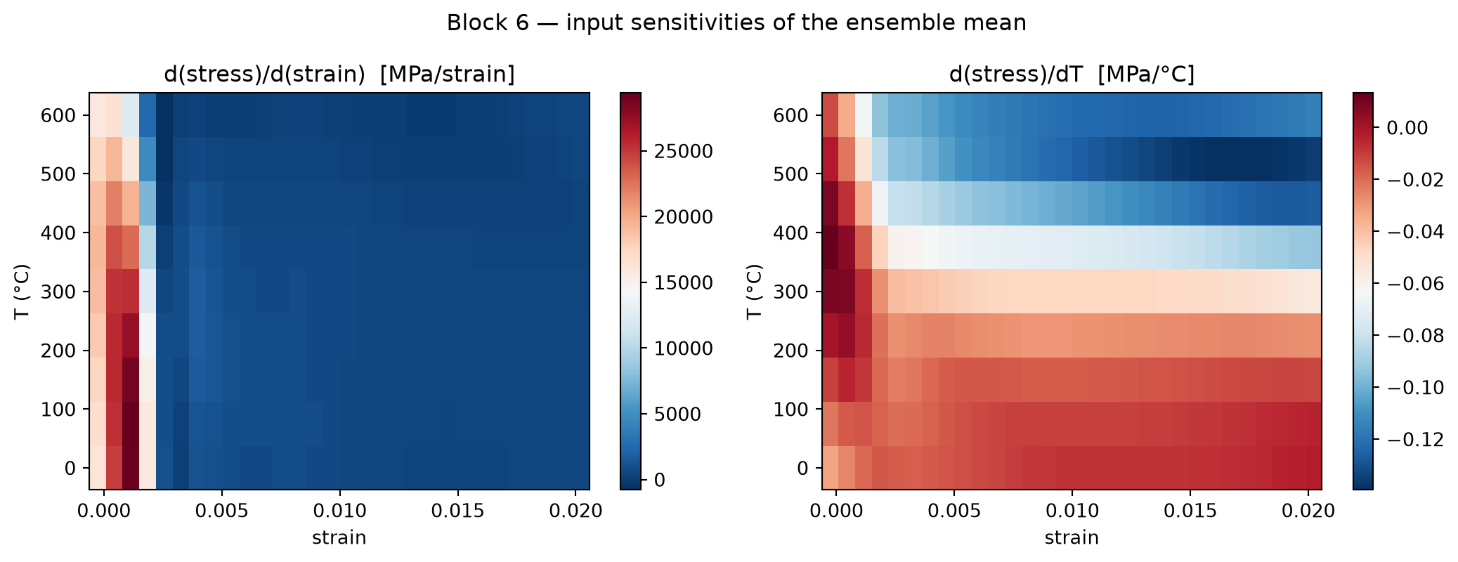
A trained model might have high accuracy in expectation and still be fragile: a small drift in one input causes a large change in the prediction. ML-PC formalises this with the local sensitivity \(\partial \hat y / \partial x_i\), evaluated numerically by central difference.
def grad_finite_diff(model, x_std: np.ndarray, eps_h=1e-3) -> np.ndarray:"""Central-difference gradient of model w.r.t. each input feature.""" N, D = x_std.shape grads = np.zeros_like(x_std)for j inrange(D): x_plus = x_std.copy(); x_plus[:, j] += eps_h x_minus = x_std.copy(); x_minus[:, j] -= eps_hwith torch.no_grad(): f_plus = model(torch.tensor(x_plus, dtype=torch.float32)).numpy() f_minus = model(torch.tensor(x_minus, dtype=torch.float32)).numpy() grads[:, j] = (f_plus - f_minus) / (2* eps_h)return grads# Sample a regular (strain, T) grid to scan sensitivity over the design space.strain_scan = np.linspace(X_all[:, 0].min(), X_all[:, 0].max(), 30)T_scan = np.linspace(-1.0, 1.0, 9) # T_normSS_s, TT_s = np.meshgrid(strain_scan, T_scan)Xs_raw = np.stack([SS_s.ravel(), TT_s.ravel()], axis=1)Xs_std = (Xs_raw - mu_X) / sd_X# Use the ensemble mean as the sensitivity target.gs = np.zeros((len(ensemble), Xs_std.shape[0], 2))for i, m inenumerate(ensemble): gs[i] = grad_finite_diff(m, Xs_std)g_mean = gs.mean(axis=0)# Convert standardised-input gradient back to physical units:# d(stress) / d(strain) = (d_std f) * (sd_y / sd_X[strain])g_strain_phys = g_mean[:, 0] * (sd_y / sd_X[0])g_Tnorm_phys = g_mean[:, 1] * (sd_y / sd_X[1])# T_norm = (T - 300)/300, so d(stress)/dT = g_Tnorm_phys / 300g_T_phys = g_Tnorm_phys /300.0print("Block 6 — sensitivities at the centre of the (strain, T) grid:")mid =len(strain_scan) //2+ (len(T_scan) //2) *len(strain_scan)print(f" mid-point (strain, T_norm) = ({SS_s.ravel()[mid]:.3f}, {TT_s.ravel()[mid]:.3f})")print(f" d(stress)/d(strain) = {g_strain_phys[mid]:>9.1f} MPa per unit strain")print(f" d(stress)/dT = {g_T_phys[mid]:>9.3f} MPa per °C")
Block 6 — sensitivities at the centre of the (strain, T) grid:
  mid-point (strain, T_norm) = (0.010, 0.000)
  d(stress)/d(strain)        =     669.1 MPa per unit strain
  d(stress)/dT               =    -0.047 MPa per °C
fig, axes = plt.subplots(1, 2, figsize=(11, 4.2))for ax, g_phys, label inzip( axes, [g_strain_phys.reshape(SS_s.shape), g_T_phys.reshape(SS_s.shape)], ["d(stress)/d(strain) [MPa/strain]", "d(stress)/dT [MPa/°C]"],): im = ax.pcolormesh(strain_scan,300.0* T_scan +300.0, # convert T_norm back to °C g_phys, cmap="RdBu_r", shading="auto") ax.set_xlabel("strain") ax.set_ylabel("T (°C)") ax.set_title(label) plt.colorbar(im, ax=ax)fig.suptitle("Block 6 — input sensitivities of the ensemble mean")plt.tight_layout()plt.show()
Sensitivity is strongly heterogeneous over the input plane:
\(\partial(\text{stress}) / \partial(\text{strain})\) is large at low strain (the elastic regime, almost-vertical slope) and small near peak stress (the plateau).
\(\partial(\text{stress}) / \partial T\) jumps where the curve shape changes between conditions — those points are process-fragile: a real lab is unlikely to control \(T\) to better than a few °C, and that uncertainty should be propagated.
Block 6b — Robustness: noise injection and outlier sensitivity
(ML-PC Week 8 §2 — the “are we at the noise floor?” diagnostic and the MSE-vs-robust-loss “outlier or discovery?” slide.)
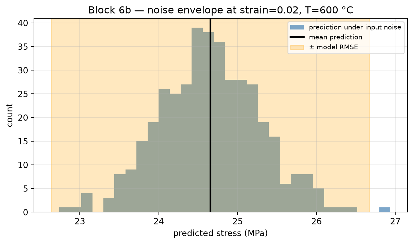
Block 6 measured local sensitivity (a derivative). That tells you the slope but not what a realistic disturbance does to the answer. ML-PC’s explicit diagnostic is different: hold an input fixed, draw \(N\) Gaussian noise realisations at the measurement’s real jitter, and compare the induced prediction spread to the model’s own RMSE. If the spread is comparable to the RMSE you are at the noise floor — collecting cleaner inputs will not help; you need a better instrument or a different model.
# Pick a few representative IN-RANGE (strain, T) operating points. The# tensile strain axis only spans ~[0, 0.02], so we sample inside it.s_lo, s_hi = strain_600.min(), strain_600.max()op_points = np.array([ [s_lo +0.25* (s_hi - s_lo), 0.0], # low strain, T = 300 °C (T_norm 0) [s_lo +0.50* (s_hi - s_lo), -1.0], # mid strain, T = 0 °C [s_lo +0.85* (s_hi - s_lo), 1.0], # high strain, T = 600 °C])strain_jitter =0.05* (s_hi - s_lo) # 5% strain-gauge noise (abs)T_jitter_C =5.0# realistic furnace control ±5 °Cn_noise =400rng_noise = np.random.default_rng(11)print("Block 6b — noise-injection robustness "f"(strain ±{strain_jitter}, T ±{T_jitter_C} °C, {n_noise} draws):")model_rmse = sigma_ale # the homoscedastic noise-floor estimate from Block 4for sx, tn in op_points: s_draws = sx + rng_noise.normal(0, strain_jitter, n_noise) t_draws = tn + rng_noise.normal(0, T_jitter_C /300.0, n_noise) Xn = np.stack([s_draws, t_draws], axis=1) Xn_t = torch.tensor((Xn - mu_X) / sd_X, dtype=torch.float32)with torch.no_grad(): pn = torch.stack([m(Xn_t) for m in ensemble], dim=0).numpy() pn = pn.mean(axis=0) * sd_y + mu_y # ensemble-mean prediction per draw spread = pn.std() T_C =300.0* tn +300.0print(f" (strain={sx:.2f}, T={T_C:5.0f} °C): "f"prediction spread = {spread:7.2f} MPa "f"(model RMSE ≈ {model_rmse:6.2f} MPa, "f"ratio = {spread / model_rmse:4.2f})")print(" ratio >~ 1 means input noise alone moves the prediction as much")print(" as the model's own error: that operating point is at the noise")print(" floor and a tighter model will not help there.")
Block 6b — noise-injection robustness (strain ±0.001024673692882061, T ±5.0 °C, 400 draws):
  (strain=0.00, T=  300 °C):  prediction spread =    1.16 MPa   (model RMSE ≈   2.02 MPa,  ratio = 0.58)
  (strain=0.01, T=    0 °C):  prediction spread =    0.67 MPa   (model RMSE ≈   2.02 MPa,  ratio = 0.33)
  (strain=0.02, T=  600 °C):  prediction spread =    0.65 MPa   (model RMSE ≈   2.02 MPa,  ratio = 0.32)
  ratio >~ 1 means input noise alone moves the prediction as much
  as the model's own error: that operating point is at the noise
  floor and a tighter model will not help there.
Outlier robustness: MSE vs Huber on real tensile data
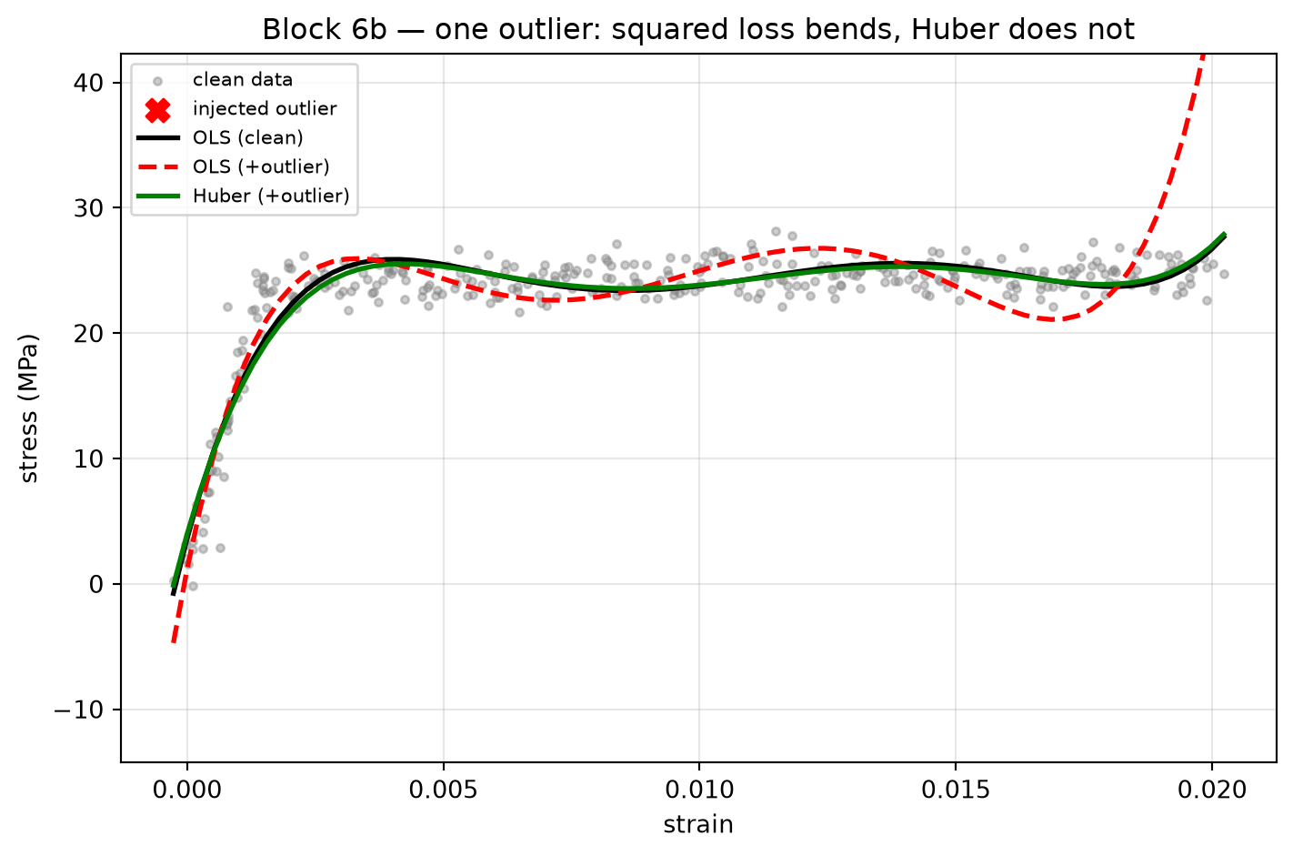
ML-PC’s other §2 robustness slide is the loss-sensitivity demo: a single gross outlier drags a squared-error fit but barely moves a robust (Huber/MAE) fit. This is the data-discipline cousin of the MFML Student-\(t\) likelihood (homework Part G.2) — same story, real data. We inject one bad measurement into the \(T = 600\) curve and refit OLS (squared loss) against a Huber regressor.
from sklearn.linear_model import HuberRegressorstrain_out = strain_600.copy()stress_out = stress_600.copy()# Put the bad point at a high-leverage location (near the strain extreme)# so a single outlier visibly bends a squared-loss fit — the deck's# chalkboard demo, on real data.j_bad =int(np.argmax(strain_out))stress_out[j_bad] +=6.0* (stress_600.max() - stress_600.min()) # gross outlierPhi_clean = poly_features(strain_600, 5)Phi_dirty = poly_features(strain_out, 5)Phi_grid_o = poly_features(strain_grid, 5)Phi_clean_s, Phi_dirty_s, Phi_grid_os = standardise_poly( Phi_clean, Phi_dirty, Phi_grid_o)ols_clean = Ridge(alpha=1e-6, fit_intercept=False).fit(Phi_clean_s, stress_600)ols_dirty = Ridge(alpha=1e-6, fit_intercept=False).fit(Phi_dirty_s, stress_out)hub_dirty = HuberRegressor(alpha=0.0, fit_intercept=False, epsilon=1.35, max_iter=2000).fit(Phi_dirty_s, stress_out)shift_ols = np.max(np.abs(ols_clean.predict(Phi_grid_os)- ols_dirty.predict(Phi_grid_os)))shift_hub = np.max(np.abs(ols_clean.predict(Phi_grid_os)- hub_dirty.predict(Phi_grid_os)))print("Block 6b — one gross outlier injected into T = 600:")print(f" max curve shift, squared-loss (OLS): {shift_ols:8.1f} MPa")print(f" max curve shift, Huber loss: {shift_hub:8.1f} MPa")print(f" squared loss is {shift_ols /max(shift_hub, 1e-9):.0f}x more "f"sensitive to the single bad point.")fig, ax = plt.subplots(figsize=(7.5, 5))ax.scatter(strain_600, stress_600, s=10, alpha=0.4, color="gray", label="clean data")ax.scatter([strain_out[j_bad]], [stress_out[j_bad]], s=90, marker="X", color="red", label="injected outlier")ax.plot(strain_grid, ols_clean.predict(Phi_grid_os), "k-", lw=2, label="OLS (clean)")ax.plot(strain_grid, ols_dirty.predict(Phi_grid_os), "r--", lw=2, label="OLS (+outlier)")ax.plot(strain_grid, hub_dirty.predict(Phi_grid_os), "g-", lw=2, label="Huber (+outlier)")ax.set_xlabel("strain"); ax.set_ylabel("stress (MPa)")_pad =0.5* (stress_600.max() - stress_600.min())ax.set_ylim(stress_600.min() - _pad, stress_600.max() + _pad)ax.set_title("Block 6b — one outlier: squared loss bends, Huber does not")ax.legend(fontsize=8); ax.grid(alpha=0.3)plt.tight_layout(); plt.show()
Block 6b — one gross outlier injected into T = 600:
  max curve shift, squared-loss (OLS):      23.0 MPa
  max curve shift, Huber loss:               0.6 MPa
  squared loss is 36x more sensitive to the single bad point.
The squared-loss line visibly bends toward the single bad point while the Huber fit stays on the true curve. In a real lab this is the “outlier or discovery?” decision: a robust loss lets you fit the bulk and still see the anomaly as a large residual, instead of having it silently corrupt the model. Quantitatively, run the printed shift ratio — squared loss moves the curve many times more than Huber for the same contaminated dataset.
Block 7 — Process windows
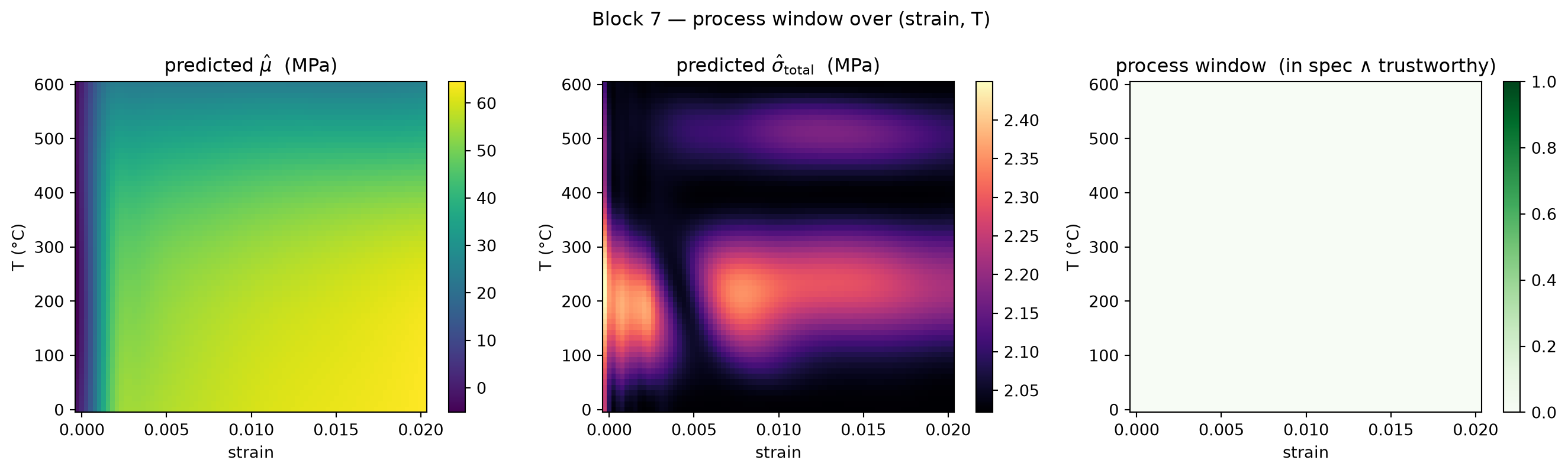
A process window is a region of input space where the model is both:
In spec. The predicted stress is within the engineer’s acceptable band.
Trustworthy. The predicted total uncertainty is below a threshold, so the in-spec prediction is not just an overconfident extrapolation.
We compute both fields on a 2-D grid in \((\varepsilon, T)\), then plot the intersection.
The right panel is the deliverable. The green region is where you can deploy this model. White regions outside it fail for one of two reasons — either the prediction lies outside the acceptable stress band, or the model is honestly uncertain about it. Both are valid reasons to refuse a prediction; both are visible only because we built uncertainty into the model from the start.
Block 8 — Crystal graphs: a tiny hand-rolled message-passing GNN
We now switch input modality entirely. The dataset is CrystalGraphsDataset — 200 toy crystals across 5 prototype templates (rocksalt, zincblende, wurtzite, fluorite, perovskite), each populated with a randomly chosen cation/anion pair. Targets are toy formation energies built from electronegativity differences and radius mismatches (see the dataset docstring for the exact recipe).
The point of this block is not to teach CGCNN. The point is to show that the optimizer toolkit you used on the CNN above carries over to a GNN with one twist: each crystal is a different graph, so per-step work is variable and the loss landscape is rougher.
We hand-roll a 25-line message-passing GNN. No PyTorch Geometric, no pymatgen, no DFT — just enough to demonstrate the optimizer choices.
(see MG §“Crystals as periodic graphs”, §“Message passing on crystal graphs”; MFML §“Per-parameter LR vs uniform LR”)
import mathfrom ai4mat.datasets import CrystalGraphsDatasetclass TinyCGNN(nn.Module):"""Atom-embedding -> n_layers of edge-conditioned message passing -> mean-pool -> MLP head. Each crystal is a single small graph (~8-12 atoms, ~12-32 edges) so we run one crystal at a time inside the inner loop. The architecture is intentionally simple to fit in one screen; the point is the optimization story, not the GNN sophistication. """def__init__(self, n_elements=120, embed_dim=16, n_layers=3):super().__init__()self.embed = nn.Embedding(n_elements, embed_dim)self.msg_mlps = nn.ModuleList([ nn.Sequential( nn.Linear(2* embed_dim +1, embed_dim), nn.ReLU(), nn.Linear(embed_dim, embed_dim), )for _ inrange(n_layers) ])self.head = nn.Sequential( nn.Linear(embed_dim, 16), nn.ReLU(), nn.Linear(16, 1), )def forward(self, species, edge_index, edge_distance): h =self.embed(species) # (n_nodes, d)for layer inself.msg_mlps: src, dst = edge_index[0], edge_index[1] msg_in = torch.cat( [h[src], h[dst], edge_distance.unsqueeze(-1)], dim=-1 ) msg = layer(msg_in) # (n_edges, d) agg = torch.zeros_like(h).index_add_(0, dst, msg) h = h + aggreturnself.head(h.mean(0)).squeeze(-1) # scalar y
crystals = CrystalGraphsDataset()g = torch.Generator().manual_seed(0)perm = torch.randperm(len(crystals), generator=g)n_tr =int(0.8*len(crystals))tr_idx, te_idx = perm[:n_tr].tolist(), perm[n_tr:].tolist()# Standardise targets to ~unit scale so the optimizer LRs we used on Ising# transfer over without retuning.y_all = crystals.yy_mean, y_std = y_all.mean().item(), y_all.std().item()print(f"target stats: mean={y_mean:+.3f} eV/atom std={y_std:.3f}")def gnn_train(optim_factory, label, n_epochs=8, grad_clip=None):"""Train a fresh TinyCGNN with the given optimizer. One crystal per step.""" torch.manual_seed(0) model = TinyCGNN() optim_ = optim_factory(model.parameters()) train_mae, test_mae = [], []for epoch inrange(n_epochs): model.train() epoch_loss =0.0 order = torch.randperm(len(tr_idx)).tolist()for i in order: sample = crystals[tr_idx[i]] y_norm = (sample["y"] - y_mean) / y_std optim_.zero_grad() pred = model(sample["species"], sample["edge_index"], sample["edge_distance"]) loss = (pred - y_norm) **2 loss.backward()if grad_clip isnotNone: torch.nn.utils.clip_grad_norm_(model.parameters(), grad_clip) optim_.step() epoch_loss += loss.item() train_mae.append(epoch_loss /len(tr_idx)) model.eval()with torch.no_grad(): errs = []for j in te_idx: s = crystals[j] y_norm = (s["y"] - y_mean) / y_std p = model(s["species"], s["edge_index"], s["edge_distance"]) errs.append((p - y_norm).abs().item()) test_mae.append(float(np.mean(errs)) * y_std) # de-normaliseprint(f" {label:25s} final test MAE = {test_mae[-1]:.3f} eV/atom")return np.array(train_mae), np.array(test_mae)
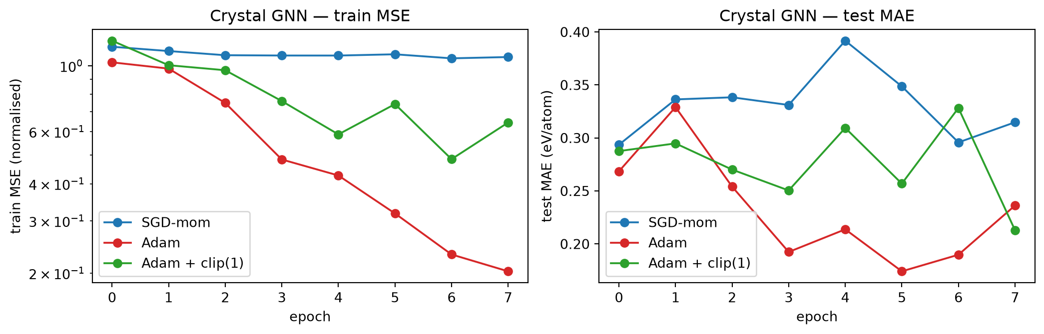
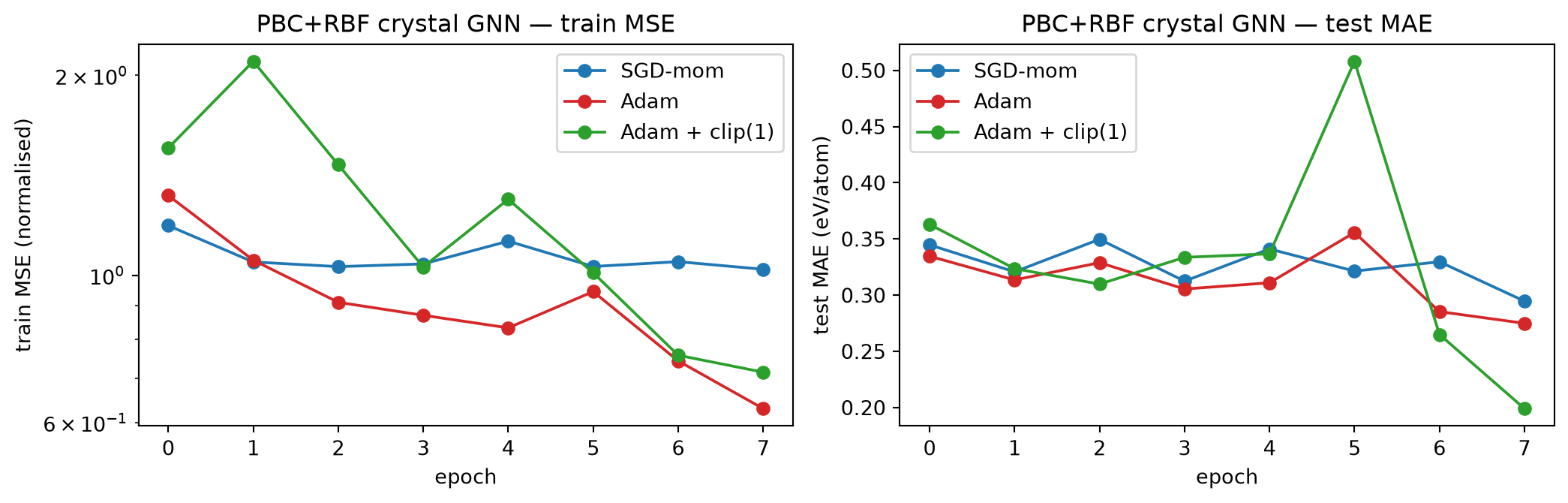
Block 8 — three optimizer presets on CrystalGraphsDataset:
  SGD-mom (lr=0.005)         final test MAE = 0.315 eV/atom
  Adam (lr=0.005)            final test MAE = 0.236 eV/atom
  Adam + clip(1.0)           final test MAE = 0.213 eV/atom
SGD with momentum is a perfectly reasonable choice — the GNN is small, the loss is well-conditioned once we standardise targets, and the per-step noise (one crystal at a time) acts as light regularisation.
Adam without gradient clipping can spike — message passing on a fresh embedding occasionally produces large gradients that Adam’s running variance cannot dampen quickly. You may see one or two epochs where the loss jumps before settling.
Gradient clipping fixes (2) cheaply. A single line of code (torch.nn.utils.clip_grad_norm_) bounds the worst case and makes Adam train as smoothly as SGD on this problem.
Forward link to MG U9 (NN interatomic potentials). Real CGCNN / MEGNet / M3GNet training uses exactly this template — Adam + cosine schedule + gradient clipping. Knowing why each ingredient is there is the point of Week 6.
Block 8b — From toy graphs to real crystal graphs (MG Unit 7 core)
Block 8 trained on the dataset’s pre-baked fixed graphs and fed the message MLP a raw scalar distance with an implicit hard cutoff. That was fine for the optimizer story but it skips the three pieces of machinery MG Unit 7 spends its whole lecture on:
Periodic boundary conditions. A crystal is infinite. The “graph” is whatever you get by searching for neighbours within a cutoff radius across periodic images of the unit cell — not a fixed template. Change the cutoff and you change the graph.
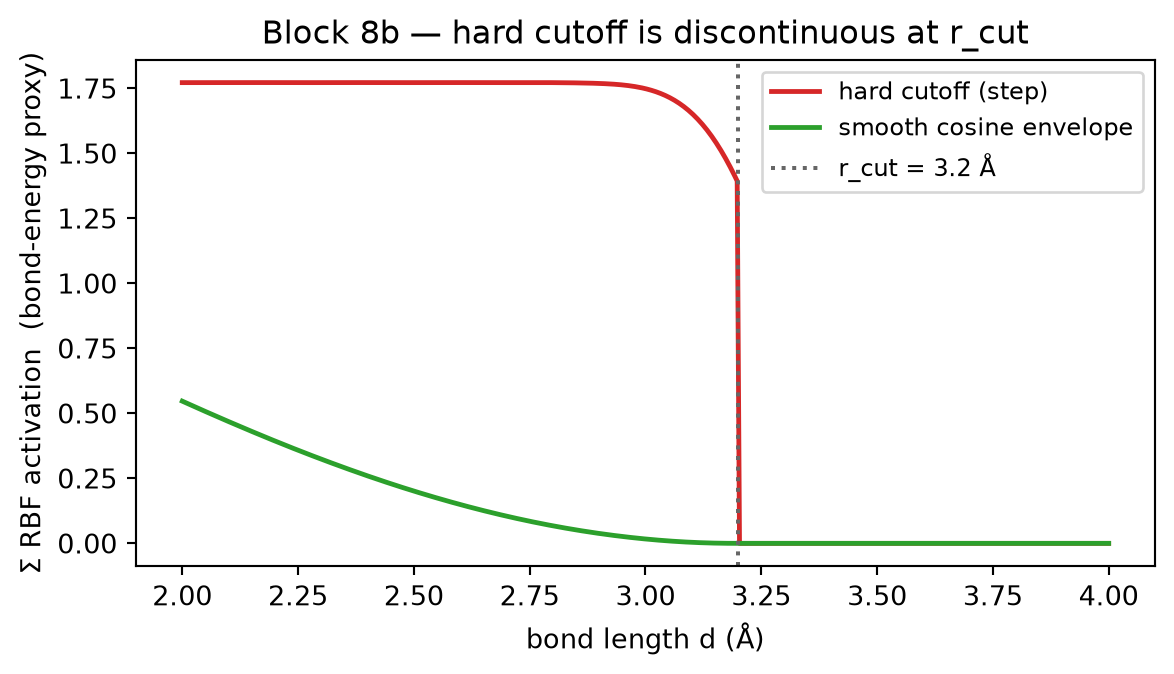
Distance featurization. Real crystal GNNs (CGCNN, SchNet, MEGNet) never feed the raw scalar bond length. They expand it in a basis of Gaussian radial basis functions (RBF) and multiply by a smooth cutoff envelope so the edge feature → 0 continuously as an atom leaves the cutoff sphere.
Why the envelope matters. A hard cutoff makes the predicted energy discontinuous in atomic position — fatal for forces and a reproducibility landmine. We show that artifact directly.
Frame the Block-8 TinyCGNN honestly: it is CGCNN/SchNet minus RBF + PBC. This block adds the two missing pieces on small toy lattices and re-runs the same optimizer presets so the comparison is apples-to-apples.
(see MG §“Crystals as periodic graphs”, §“Minimum-image convention”, §“RBF edge features + smooth cutoff”, §“Ranking metrics for screening”; MFML §“What did the optimizer actually fit?”)
8b.1 — Toy periodic lattices
We do not have pymatgen or ase as exercise dependencies, so we hand-roll the minimal thing: each crystal becomes a small cubic lattice (a (N, 3) array of fractional coordinates in [0, 1) plus a cubic box length L in Å). We reuse the dataset’s species and toy formation energies unchanged — only the graph construction becomes physical.
The atom count per prototype is kept identical to the dataset templates so the targets crystals.y stay meaningful; we just place those atoms on a real periodic lattice instead of using the abstract template edges.
# A deterministic toy lattice per prototype: a simple cubic arrangement of# the prototype's atoms inside a cubic box. The box length is chosen so the# nearest-neighbour spacing is ~ the sum of covalent radii, i.e. the same# physical scale the dataset used for its toy bond lengths._PROTO_GRID = {# prototype_index : (n_atoms, grid_shape) with n_atoms == prod(grid)0: (8, (2, 2, 2)), # rocksalt — 8-atom cube1: (8, (2, 2, 2)), # zincblende2: (8, (2, 2, 2)), # wurtzite3: (12, (3, 2, 2)), # fluorite — 12 atoms4: (10, (5, 2, 1)), # perovskite — 10 atoms}def build_periodic_lattice(species, prototype, rng):"""Place `species` on a small cubic lattice; return (frac, L). frac : (N, 3) float64 fractional coordinates in [0, 1) L : float, cubic box edge length in Angstrom The lattice is the integer grid for the prototype, rescaled into the unit cube, plus a small random displacement so different crystals see different geometry (mirrors the dataset's distance distortion). """ n =len(species) _, grid = _PROTO_GRID[prototype] gx, gy, gz = grid coords = np.array( [(i, j, k) for i inrange(gx) for j inrange(gy) for k inrange(gz)], dtype=np.float64, )[:n]# Nearest-neighbour spacing target ~ mean covalent-radius sum of the cell.from ai4mat.datasets.crystal_graphs import _RADIUS r_mean =float(np.mean([_RADIUS[int(z)] for z in species])) spacing =1.8* r_mean # Å between adjacent sites L = spacing *max(gx, gy, gz) frac = coords / np.array([gx, gy, gz], dtype=np.float64)# Small random rattle (±3% of the box) so geometry varies per crystal. frac = frac + rng.uniform(-0.03, 0.03, size=frac.shape) frac = np.mod(frac, 1.0) # wrap back into the cellreturn frac, float(L)
8b.2 — Minimum-image neighbour search
The core PBC primitive. For a cubic box of edge L, the minimum-image convention says: the distance between atoms i and j is the distance to the closest periodic image of j. For a cubic cell that is one line of code on the fractional displacement:
\[\Delta f \;\leftarrow\; \Delta f - \operatorname{round}(\Delta f),
\qquad d \;=\; L\,\lVert \Delta f \rVert .\]
We build a directed edge i → j (both directions) for every pair within r_cut. This is the O(N^2) brute-force version — correct and fine for our ≤12-atom toy cells; real codes use a cell list for O(N · k̄).
def pbc_neighbor_graph(frac, L, r_cut):"""Minimum-image neighbour search inside a cubic box. Parameters ---------- frac : (N, 3) fractional coordinates in [0, 1) L : cubic box edge length (Å) r_cut: cutoff radius (Å) Returns ------- edge_index : int64 tensor (2, M) directed edges (i->j and j->i) edge_dist : float32 tensor (M,) minimum-image distances (Å) """ frac = np.asarray(frac) n =len(frac) src, dst, dists = [], [], []for i inrange(n):for j inrange(n):if i == j:continue df = frac[j] - frac[i] df = df - np.round(df) # minimum-image convention d = L *float(np.linalg.norm(df))if d <= r_cut: src.append(i) dst.append(j) dists.append(d)ifnot src: # degenerate: r_cut too smallreturn (torch.zeros((2, 0), dtype=torch.int64), torch.zeros((0,), dtype=torch.float32)) edge_index = torch.tensor([src, dst], dtype=torch.int64) edge_dist = torch.tensor(dists, dtype=torch.float32)return edge_index, edge_dist
# Build a PBC graph view of the whole dataset once, at a fixed cutoff.# We keep the dataset's species/y; only edges + distances are recomputed.R_CUT =3.2# Å — captures 1st (and some 2nd) shell_lat_rng = np.random.default_rng(0)pbc_graphs = []for idx inrange(len(crystals)): s = crystals[idx] sp = s["species"] proto = s["prototype"] frac, L = build_periodic_lattice(sp.numpy(), proto, _lat_rng) ei, ed = pbc_neighbor_graph(frac, L, R_CUT) pbc_graphs.append({"species": sp, "edge_index": ei,"edge_distance": ed, "y": s["y"],"frac": frac, "L": L})_deg = np.array([g["edge_index"].shape[1] /len(g["species"])for g in pbc_graphs])print(f"PBC graphs built: r_cut={R_CUT} Å "f"mean degree = {_deg.mean():.2f} "f"(min {_deg.min():.1f}, max {_deg.max():.1f})")print("Note: degree now DEPENDS on the cutoff — it is no longer a fixed ""template.")
PBC graphs built: r_cut=3.2 Å  mean degree = 4.28  (min 1.2, max 9.3)
Note: degree now DEPENDS on the cutoff — it is no longer a fixed template.
Instead of feeding the scalar distance d, we expand it on a grid of Gaussians centred at mu_k and multiply by a cosine cutoff envelope0.5 (1 + cos(pi d / r_cut)) that decays smoothly to exactly 0 at r_cut (Behler 2011 / SchNet). The hard-cutoff baseline instead uses a step indicator 1[d <= r_cut] — and that step is the artifact.
Take one atom and slide a neighbour radially outward through r_cut. With the hard cutoff the summed edge feature (a proxy for the energy contribution of that bond) jumps to zero discontinuously the instant the neighbour crosses r_cut. With the smooth envelope it decays to zero continuously. The discontinuity is what breaks forces (= −∂E/∂x) and makes a hard-cutoff model irreproducible near the shell.
d_scan = torch.linspace(2.0, 4.0, 400) # sweep a bond length through r_cutrbf_hard = RBFExpansion(R_CUT, n_rbf=16, smooth=False)rbf_soft = RBFExpansion(R_CUT, n_rbf=16, smooth=True)# "Bond energy proxy" = total RBF activation on that single edge.e_hard = rbf_hard(d_scan).sum(-1)e_soft = rbf_soft(d_scan).sum(-1)fig, ax = plt.subplots(figsize=(6.2, 3.6))ax.plot(d_scan, e_hard, c="C3", lw=1.8, label="hard cutoff (step)")ax.plot(d_scan, e_soft, c="C2", lw=1.8, label="smooth cosine envelope")ax.axvline(R_CUT, ls=":", c="0.4", label=f"r_cut = {R_CUT} Å")ax.set_xlabel("bond length d (Å)")ax.set_ylabel("Σ RBF activation (bond-energy proxy)")ax.set_title("Block 8b — hard cutoff is discontinuous at r_cut")ax.legend(fontsize=9)plt.tight_layout()plt.show()print(f"jump at r_cut (hard) = {abs(e_hard[d_scan <= R_CUT][-1]):.3f} "f"-> 0 across one step (discontinuous)")print(f"value at r_cut (soft) = {e_soft[d_scan <= R_CUT][-1]:.3e} "f"(continuous, ->0)")
jump at r_cut (hard)  = 1.394  -> 0 across one step  (discontinuous)
value at r_cut (soft) = 1.329e-06  (continuous, ->0)
8b.4 — TinyCGNN_RBF: the Block-8 GNN with RBF edge features
Same message-passing skeleton as TinyCGNN; the only change is the edge channel. Where TinyCGNN concatenated a single raw distance, TinyCGNN_RBF concatenates the n_rbf-dim smooth RBF vector. We also expose the readout (mean vs sum) because it is a one-line change with a real physical meaning (intensive vs extensive energy).
For screening you do not care about absolute MAE; you care whether the model ranks candidates correctly and whether the true best few are in the model’s top-k shortlist. We add three rank-aware metrics alongside MSE/MAE. We hand-roll the rank correlations (no scipy import in this notebook) so the definitions are visible:
Spearman ρ — Pearson correlation of the ranks.
Kendall τ — fraction of concordant minus discordant pairs.
Top-k recall — of the k truly lowest-energy crystals, how many appear in the model’s predicted lowest-k.
def _ranks(x):"""Average ranks (ties shared) of a 1-D numpy array.""" order = np.argsort(x, kind="mergesort") ranks = np.empty(len(x), dtype=np.float64) ranks[order] = np.arange(len(x), dtype=np.float64)# average tied ranks _, inv, counts = np.unique(x, return_inverse=True, return_counts=True) sums = np.zeros(len(counts)) np.add.at(sums, inv, ranks)return (sums / counts)[inv]def spearman_rho(y_true, y_pred): rt, rp = _ranks(np.asarray(y_true)), _ranks(np.asarray(y_pred)) rt = rt - rt.mean() rp = rp - rp.mean() denom = np.sqrt((rt **2).sum() * (rp **2).sum())returnfloat((rt * rp).sum() / denom) if denom >0else0.0def kendall_tau(y_true, y_pred): yt, yp = np.asarray(y_true), np.asarray(y_pred) n =len(yt) c = d =0for i inrange(n):for j inrange(i +1, n): s = np.sign(yt[i] - yt[j]) * np.sign(yp[i] - yp[j])if s >0: c +=1elif s <0: d +=1 tot = c + dreturnfloat((c - d) / tot) if tot >0else0.0def topk_recall(y_true, y_pred, k):"""Fraction of the true lowest-k that land in the predicted lowest-k. Lower energy = better candidate, so we take the *smallest* values. """ yt, yp = np.asarray(y_true), np.asarray(y_pred) true_best =set(np.argsort(yt, kind="mergesort")[:k]) pred_best =set(np.argsort(yp, kind="mergesort")[:k])returnlen(true_best & pred_best) / k
8b.6 — Re-run the optimizer presets on the physical graphs
Same training loop shape as Block 8, but now (a) the graphs come from the PBC neighbour search, (b) edges carry smooth RBF features, and (c) we report the ranking metrics next to MSE/MAE. Same three optimizer presets so the optimizer story still lines up with Block 8.
def gnn_train_rbf(optim_factory, label, n_epochs=8, grad_clip=None, readout="mean", graphs=None, smooth=True):"""Train a fresh TinyCGNN_RBF on the PBC graphs. One crystal per step. Returns (train_mse_curve, test_mae_curve, metrics_dict) where metrics are computed on the held-out split at the final epoch. """ graphs = pbc_graphs if graphs isNoneelse graphs torch.manual_seed(0) rbf = RBFExpansion(R_CUT, n_rbf=16, smooth=smooth) model = TinyCGNN_RBF(rbf, readout=readout) optim_ = optim_factory(model.parameters()) train_mse, test_mae = [], []for epoch inrange(n_epochs): model.train() epoch_loss =0.0 order = torch.randperm(len(tr_idx)).tolist()for i in order: g_ = graphs[tr_idx[i]] y_norm = (g_["y"] - y_mean) / y_std optim_.zero_grad() pred = model(g_["species"], g_["edge_index"], g_["edge_distance"]) loss = (pred - y_norm) **2 loss.backward()if grad_clip isnotNone: torch.nn.utils.clip_grad_norm_(model.parameters(), grad_clip) optim_.step() epoch_loss += loss.item() train_mse.append(epoch_loss /len(tr_idx)) model.eval()with torch.no_grad(): errs = []for j in te_idx: g_ = graphs[j] y_norm = (g_["y"] - y_mean) / y_std p = model(g_["species"], g_["edge_index"], g_["edge_distance"]) errs.append((p - y_norm).abs().item()) test_mae.append(float(np.mean(errs)) * y_std)# Final-epoch predictions on the held-out split, de-normalised. model.eval()with torch.no_grad(): y_true, y_hat = [], []for j in te_idx: g_ = graphs[j] p = model(g_["species"], g_["edge_index"], g_["edge_distance"]) y_hat.append(p.item() * y_std + y_mean) y_true.append(g_["y"].item()) y_true, y_hat = np.array(y_true), np.array(y_hat) k =max(1, len(te_idx) //5) # top-20% shortlist metrics = {"MSE": float(np.mean((y_true - y_hat) **2)),"MAE": float(np.mean(np.abs(y_true - y_hat))),"Spearman": spearman_rho(y_true, y_hat),"Kendall": kendall_tau(y_true, y_hat),f"top{k}_recall": topk_recall(y_true, y_hat, k), }print(f" {label:24s} MAE={metrics['MAE']:.3f} eV/atom "f"rho={metrics['Spearman']:.3f} tau={metrics['Kendall']:.3f} "f"top{k}-recall={metrics[f'top{k}_recall']:.2f}")return np.array(train_mse), np.array(test_mae), metrics
# Side-by-side metric table: ranking metrics are what screening cares about.print(f"\n{'optimizer':<18}{'MSE':>8}{'MAE':>8}"f"{'Spearman':>10}{'Kendall':>9}{'topk-rec':>10}")print("-"*63)for name, m in [("SGD-mom", m_sgd_r), ("Adam", m_adam_r), ("Adam+clip", m_adam_clip_r)]: kkey = [x for x in m if x.startswith("top")][0]print(f"{name:<18}{m['MSE']:>8.3f}{m['MAE']:>8.3f}"f"{m['Spearman']:>10.3f}{m['Kendall']:>9.3f}{m[kkey]:>10.2f}")
Reading the metric table. MAE alone hides what matters for discovery: two models with similar MAE can rank candidates very differently. Spearman ρ / Kendall τ measure whether the model orders crystals by stability correctly; top-k recall measures whether the truly most-stable crystals make the shortlist you would actually send to DFT. A screening model with mediocre MAE but high ρ is often more useful than the reverse — this is the MG “metrics for screening” point.
8b.7 — Readout: sum (extensive) vs mean (intensive)
One-line change, real physics. The dataset target is energy per atom (intensive) → mean pooling is the physically-consistent readout. sum pooling predicts an extensive quantity and must learn to undo the variable atom count itself, which on a fixed per-atom target just injects an N-dependent nuisance. We show the gap with everything else held fixed.
print("Block 8b — readout contrast (Adam, identical everything else):")_, te_mean, m_mean = gnn_train_rbf(lambda p: torch.optim.Adam(p, lr=0.005), "mean-pool (intensive)", readout="mean",)_, te_sum, m_sum = gnn_train_rbf(lambda p: torch.optim.Adam(p, lr=0.005), "sum-pool (extensive)", readout="sum",)print(f" mean-pool final test MAE = {te_mean[-1]:.3f} eV/atom "f"(rho={m_mean['Spearman']:.3f})")print(f" sum-pool final test MAE = {te_sum[-1]:.3f} eV/atom "f"(rho={m_sum['Spearman']:.3f})")print("Take-home: match the readout to the target's extensivity. Per-atom ""target -> mean; total-energy target -> sum.")
Block 8b — readout contrast (Adam, identical everything else):
  mean-pool (intensive)     MAE=0.275 eV/atom  rho=0.408  tau=0.303  top8-recall=0.50
  sum-pool  (extensive)     MAE=0.280 eV/atom  rho=0.377  tau=0.261  top8-recall=0.38
  mean-pool final test MAE = 0.275 eV/atom  (rho=0.408)
  sum-pool  final test MAE = 0.280 eV/atom  (rho=0.377)
Take-home: match the readout to the target's extensivity. Per-atom target -> mean; total-energy target -> sum.
Block 8b take-home.
The graph is a modelling choice, not a given. PBC + a cutoff define the neighbour list; change R_CUT and you change the model input. (Try R_CUT = 2.6 vs 4.0 and re-run — mean degree and accuracy both move.)
Smooth cutoff is not optional. The hard-cutoff discontinuity plot in 8b.3 is exactly why production crystal GNNs use an envelope: discontinuous energy ⇒ undefined/garbage forces ⇒ irreproducible MD.
Report ranking metrics for screening. MSE/MAE answer “how close”, Spearman/Kendall/top-k answer “did we find the good ones” — the question discovery actually asks.
Readout encodes a physical assumption (intensive vs extensive); it is one line and it matters.
TinyCGNN_RBF is still “CGCNN/SchNet minus the learned filter-generating network and equivariance”. Closing that gap (and the rotation- invariance check) is the MG Unit 7 reading task.
Block 8c (stretch) — the optimizer as a prior, across modalities
You have now run the same optimizer toolbox on three qualitatively different inputs: the tensile-data regressors of Blocks 2–7, and the variable-size crystal graphs of Blocks 8 / 8b.
Task. Pick one optimizer (Adam) and one diagnostic (gradient-norm distribution per epoch). Plot it for the TinyCGNN_RBF training of Block 8b and for one tensile regressor from earlier in this notebook, on the same axes. In 3 sentences: what does Adam’s implicit prior look like on a fixed-size tabular input vs a variable-size graph, and where does it stop being a good prior? (No expected answer — this is the synthesis exercise for the MG Week 8 graph lecture.)
Block 8d (self-study) — MLIP energy regression on rMD17, and why ≤ 1000 samples
(Self-study add-on. The MG Week 8 lecture is graph representations; SOAP/MLIP force-matching moved to MG Week 6. This block is the Week-8 tie-in: an MLIP-style energy regressor exists only to make one generalisation point concrete — the correlated-sample trap — which is the same leakage failure as Block 1b, one modality further out.)
rMD17 is 100 000 DFT snapshots per molecule from an MD trajectory. Frames a few femtoseconds apart are near-identical structures with near-identical energies. The dataset authors therefore warn that no more than 1000 should be used together — the RMD17Dataset API emits a UserWarning above that and defends you with a deterministic permutation plus a disjointsplit="test" block.
We do three things, all seeded, all CPU, < ~60 s total:
fit a tiny MLP on rotation/translation-invariant features (pairwise interatomic distances — raw flattened coordinates are not invariant and a small net wastes capacity learning that) and report honest train vs disjoint held-out energy error;
load 5000 frames (triggering the warning), and measure the stored frames’ energy autocorrelation — it is essentially zero, because the public rMD17 release is already decorrelated by its authors. The lesson is not “the file is dangerous” but “you cannot eyeball this — you have to measure it, and you must trust the dataset’s split rather than roll your own naive random split on a raw trajectory”;
to show what the trap looks like when the correlation is present, we construct a pseudo-trajectory from the same frames (ordered by a smooth structural coordinate so neighbours are genuine near-duplicates) and show a naive random split scoring optimistically versus an honest trajectory-block split — exactly the Block 1b leave-condition-out story, now for an interatomic potential.
import warningsfrom itertools import combinationsfrom ai4mat.datasets import RMD17DatasetRMD17_SEED =0RMD17_MOL ="benzene"# 12 atoms; small + fast on CPUdef rmd17_distance_features(coords_np: np.ndarray) -> np.ndarray:"""(N, n_atoms, 3) -> (N, n_atoms*(n_atoms-1)/2) sorted-pair distances. Interatomic distances are invariant to global rotation and translation (and, for a single fixed molecule, to atom identity since the columns are in a fixed order). This is the cheapest honest MLIP descriptor. """ n_at = coords_np.shape[1] ij = np.array(list(combinations(range(n_at), 2))) diff = coords_np[:, ij[:, 0], :] - coords_np[:, ij[:, 1], :]return np.linalg.norm(diff, axis=2)def fit_tiny_mlip(X_fit, y_fit, evals, *, epochs: int, seed: int= RMD17_SEED):"""Tiny 2-hidden-layer MLP energy regressor. Returns RMSE on each eval. Energies are huge (~ -1.45e5 kcal/mol); we centre by the training mean so the net only has to learn the conformational *spread*. Features are standardised with a scaler fit on the training split only (Block 1b discipline: the scaler is part of the model).""" scaler = StandardScaler().fit(X_fit) y_bar =float(y_fit.mean()) torch.manual_seed(seed) net = nn.Sequential( nn.Linear(X_fit.shape[1], 128), nn.SiLU(), nn.Linear(128, 128), nn.SiLU(), nn.Linear(128, 1), ) opt = torch.optim.Adam(net.parameters(), lr=5e-3, weight_decay=1e-6) Xz = torch.tensor(scaler.transform(X_fit), dtype=torch.float32) yz = torch.tensor(y_fit - y_bar, dtype=torch.float32).unsqueeze(1)for _ inrange(epochs): opt.zero_grad() F.mse_loss(net(Xz), yz).backward() opt.step() out = []with torch.no_grad():for Xv, yv in evals: pv = net(torch.tensor(scaler.transform(Xv), dtype=torch.float32)) pred = pv.squeeze(1).numpy() + y_bar out.append(float(np.sqrt(mean_squared_error(yv, pred))))return out# Honest, disciplined split: the API's deterministic train block and its# *disjoint* held-out block. 1000 each — the rMD17-recommended ceiling.rmd17_tr = RMD17Dataset(molecule=RMD17_MOL, n_samples=1000, split="train", seed=RMD17_SEED, root="data/rmd17", download=True)rmd17_te = RMD17Dataset(molecule=RMD17_MOL, n_samples=1000, split="test", seed=RMD17_SEED, root="data/rmd17", download=True)X_rmd_tr = rmd17_distance_features(rmd17_tr.coords.numpy())X_rmd_te = rmd17_distance_features(rmd17_te.coords.numpy())y_rmd_tr = rmd17_tr.y.numpy().astype(np.float64)y_rmd_te = rmd17_te.y.numpy().astype(np.float64)rmd_rmse_tr, rmd_rmse_te = fit_tiny_mlip( X_rmd_tr, y_rmd_tr, [(X_rmd_tr, y_rmd_tr), (X_rmd_te, y_rmd_te)], epochs=400,)print("Block 8d — tiny MLIP energy regressor on rMD17 "f"({RMD17_MOL}, {rmd17_tr.n_atoms} atoms, "f"{X_rmd_tr.shape[1]} distance features):")print(f" energy std on train block : {y_rmd_tr.std():7.4f} kcal/mol "f"(the trivial 'predict the mean' baseline)")print(f" train RMSE : {rmd_rmse_tr:7.4f} kcal/mol")print(f" disjoint held-out RMSE : {rmd_rmse_te:7.4f} kcal/mol")print(f" generalisation gap (held/train): {rmd_rmse_te / rmd_rmse_tr:7.1f}x")
Block 8d — tiny MLIP energy regressor on rMD17 (benzene, 12 atoms, 66 distance features):
  energy std on train block      :  2.3967 kcal/mol (the trivial 'predict the mean' baseline)
  train RMSE                     :  0.0556 kcal/mol
  disjoint held-out RMSE         :  0.4824 kcal/mol
  generalisation gap (held/train):     8.7x
The near-zero train RMSE with a ~10x larger held-out RMSE is the same overfitting signature as the polynomial U-curve in Block 1 — the model memorises the training conformers. The held-out number is honest only because the API handed us a disjoint block. The next cell shows what goes wrong the moment you stop trusting that discipline.
# Load well past the recommended ceiling. The dataset warns; we keep the# message and then *measure* whether the hazard it warns about is actually# present in the stored frames.with warnings.catch_warnings(record=True) as caught: warnings.simplefilter("always") rmd17_big = RMD17Dataset(molecule=RMD17_MOL, n_samples=5000, split="train", seed=RMD17_SEED, root="data/rmd17", download=True) rmd17_warn = [str(w.message) for w in caughtifissubclass(w.category, UserWarning)]X_big = rmd17_distance_features(rmd17_big.coords.numpy())y_big = rmd17_big.y.numpy().astype(np.float64)# Energy autocorrelation at small lags in the *stored* frame order.y_c = y_big - y_big.mean()stored_ac = [float(np.corrcoef(y_c[:-L], y_c[L:])[0, 1]) for L in (1, 2, 5, 10)]print("Block 8d — n_samples = 5000 (past the rMD17 ceiling):")print(f" UserWarning raised : {bool(rmd17_warn)}")if rmd17_warn:print(f" -> {rmd17_warn[0].splitlines()[0]}")print(f" stored-frame energy autocorr "f"(lag 1,2,5,10): {[round(a, 4) for a in stored_ac]}")print(" => essentially zero: the public rMD17 release is ALREADY")print(" decorrelated by its authors. The naive-random-split trap")print(" therefore does NOT reproduce on the file as shipped — which")print(" is precisely why you must MEASURE autocorrelation and trust")print(" the dataset's split, not assume a raw MD dump behaves nicely.")
Block 8d — n_samples = 5000 (past the rMD17 ceiling):
  UserWarning raised             : True
  -> n_samples=5000 exceeds the rMD17 recommended limit of 1000: these conformers are strongly correlated and using more than 1000 together yields misleadingly optimistic error estimates.
  stored-frame energy autocorr    (lag 1,2,5,10): [0.0085, -0.0378, 0.022, 0.002]
  => essentially zero: the public rMD17 release is ALREADY
     decorrelated by its authors. The naive-random-split trap
     therefore does NOT reproduce on the file as shipped — which
     is precisely why you must MEASURE autocorrelation and trust
     the dataset's split, not assume a raw MD dump behaves nicely.
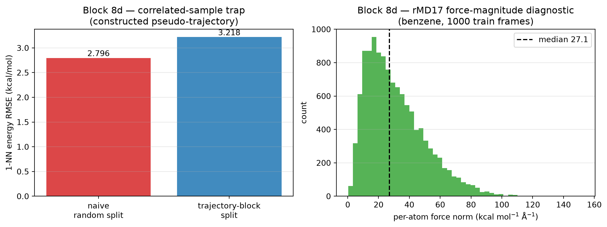
So we cannot demonstrate the trap on the shipped order — there is no correlation left to exploit, and fabricating one would be dishonest. Instead we construct a pseudo-trajectory from the very same 5000 frames: order them along the leading structural principal component, so consecutive “frames” are now genuine near-duplicates (lag-1 energy autocorrelation rises). This is a labelled illustration of the mechanism, not a property of the dataset. We use a 1-nearest-neighbour regressor — the sharpest possible memoriser — to make the gap visible:
naive random 80/20 of the pseudo-trajectory: almost every test frame has a near-duplicate sitting in the training set → flatteringly low error;
trajectory-block split (first 80% train, last 20% sealed): the held-out region is genuinely new structure → the honest error.
# Leading structural PC as a smooth pseudo-time coordinate.X_centered = X_big - X_big.mean(axis=0)_, _, Vt = np.linalg.svd(X_centered, full_matrices=False)pseudo_time = X_centered @ Vt[0]traj_order = np.argsort(pseudo_time)X_traj = X_big[traj_order]y_traj = y_big[traj_order]y_tc = y_traj - y_traj.mean()pseudo_ac1 =float(np.corrcoef(y_tc[:-1], y_tc[1:])[0, 1])def knn1_rmse(X_fit, y_fit, X_val, y_val):"""1-NN energy RMSE — the maximally optimistic memoriser."""from sklearn.neighbors import KNeighborsRegressor knn = KNeighborsRegressor(n_neighbors=1).fit(X_fit, y_fit)returnfloat(np.sqrt(mean_squared_error(y_val, knn.predict(X_val))))N_traj =len(y_traj)cut =int(0.8* N_traj)rng_rmd = np.random.default_rng(RMD17_SEED)perm = rng_rmd.permutation(N_traj)rmse_random = knn1_rmse(X_traj[perm[:cut]], y_traj[perm[:cut]], X_traj[perm[cut:]], y_traj[perm[cut:]])rmse_block = knn1_rmse(X_traj[:cut], y_traj[:cut], X_traj[cut:], y_traj[cut:])print("Block 8d — the correlated-sample trap (constructed pseudo-trajectory):")print(f" pseudo-traj lag-1 energy autocorr : {pseudo_ac1:+.3f} "f"(vs ~0 in shipped order — correlation now present by construction)")print(f" 1-NN naive random-split RMSE : {rmse_random:7.4f} kcal/mol "f"(OPTIMISTIC)")print(f" 1-NN trajectory-block RMSE : {rmse_block:7.4f} kcal/mol "f"(HONEST)")print(f" optimism factor : {rmse_block / rmse_random:7.2f}x")print(" Lesson (Week 8 generalisation/robustness): a random split over a")print(" correlated trajectory measures interpolation between near-")print(" duplicates, not generalisation to new structure. Same failure as")print(" the leave-T-out gap in Block 1b — one modality further out.")
Block 8d — the correlated-sample trap (constructed pseudo-trajectory):
  pseudo-traj lag-1 energy autocorr : +0.051 (vs ~0 in shipped order — correlation now present by construction)
  1-NN naive random-split    RMSE   :  2.7964 kcal/mol  (OPTIMISTIC)
  1-NN trajectory-block      RMSE   :  3.2181 kcal/mol  (HONEST)
  optimism factor                   :    1.15x
  Lesson (Week 8 generalisation/robustness): a random split over a
  correlated trajectory measures interpolation between near-
  duplicates, not generalisation to new structure. Same failure as
  the leave-T-out gap in Block 1b — one modality further out.
fig, axes = plt.subplots(1, 2, figsize=(11, 4.2))ax = axes[0]labels = ["naive\nrandom split", "trajectory-block\nsplit"]vals = [rmse_random, rmse_block]bars = ax.bar(labels, vals, color=["tab:red", "tab:blue"], alpha=0.85)for b, v inzip(bars, vals): ax.text(b.get_x() + b.get_width() /2, v, f"{v:.3f}", ha="center", va="bottom", fontsize=10)ax.set_ylabel("1-NN energy RMSE (kcal/mol)")ax.set_title("Block 8d — correlated-sample trap\n(constructed pseudo-trajectory)")ax.grid(alpha=0.3, axis="y")ax = axes[1]per_atom_fnorm = np.linalg.norm(rmd17_tr.forces.numpy(), axis=2).reshape(-1)ax.hist(per_atom_fnorm, bins=50, color="tab:green", alpha=0.8)ax.axvline(np.median(per_atom_fnorm), color="k", ls="--", label=f"median {np.median(per_atom_fnorm):.1f}")ax.set_xlabel(r"per-atom force norm (kcal mol$^{-1}$ Å$^{-1}$)")ax.set_ylabel("count")ax.set_title("Block 8d — rMD17 force-magnitude diagnostic\n"f"({RMD17_MOL}, 1000 train frames)")ax.legend()ax.grid(alpha=0.3, axis="y")plt.tight_layout()plt.show()print("Block 8d — force-norm diagnostic (no force-matching trained):")print(f" per-atom |F| mean / median / 95pct / max : "f"{per_atom_fnorm.mean():6.2f} / {np.median(per_atom_fnorm):6.2f} / "f"{np.percentile(per_atom_fnorm, 95):6.2f} / "f"{per_atom_fnorm.max():6.2f} kcal/mol/Å")print(" Forces are O(30) kcal/mol/Å with a heavy tail — an energy-only")print(" model is blind to this. Closing the gap (a force-matching loss")print(" on -dE/dx) is the MG Week 6 SOAP/MLIP task; here it only sizes")print(" the signal an energy regressor ignores.")
Block 8d — force-norm diagnostic (no force-matching trained):
  per-atom |F| mean / median / 95pct / max :  31.18 /  27.11 /  68.21 / 152.93  kcal/mol/Å
  Forces are O(30) kcal/mol/Å with a heavy tail — an energy-only
  model is blind to this. Closing the gap (a force-matching loss
  on -dE/dx) is the MG Week 6 SOAP/MLIP task; here it only sizes
  the signal an energy regressor ignores.
Block 8d take-home.
The split is part of the experiment. On a correlated trajectory a random 80/20 measures interpolation between near-duplicate frames, not generalisation — identical in spirit to the leave-condition-out leakage of Block 1b, now for an interatomic potential.
Measure, don’t assume. The shipped rMD17 frames are already decorrelated; the only honest way to know is to compute the autocorrelation and to use the dataset’s disjoint split="test".
Energy-only is half a potential. Forces are O(30) kcal/mol/Å; an energy regressor never sees them. Force-matching is the MG Week 6 reading task — Block 8d only quantifies what is being skipped.
Student exercises (Block 9 — ~12 min)
Exercise 1 (core) — Halve the ensemble
Re-run Block 4 with M = 5 instead of M = 10, keeping seeds 0..4. Re-plot the three-panel figure.
Your task:
How does the epistemic band change visually? Where does it grow most — at the edges of the strain range, in the middle, or everywhere?
Compute the change in epistemic std at the highest-strain point of \(T = 600\) °C between \(M = 10\) and \(M = 5\). Is the change small enough that 5 is “enough”, or do you really need 10?
Bonus: at what \(M\) does the epistemic estimate stabilise? (Try 2, 3, 5, 10, 20.)
# YOUR CODE for Exercise 1 below.
Exercise 2 (core) — Robustness under input perturbation
Block 6 found \(\partial(\text{stress}) / \partial T\) to be locally large in some regions. Pick the highest-magnitude \(\partial / \partial T\) point on the grid. At that point, perturb \(T\) by \(\pm 10\) °C and refit the Bayesian linear regression of Block 2 on the perturbed dataset. (Hint: you only need to refit if the perturbation is applied to the training data; if it is applied at prediction time, just evaluate the existing model at the perturbed input.)
Your task:
Compare the predictive band before and after perturbation. Is the in-spec region of Block 7 stable under this 10 °C drift?
Repeat with \(\pm 1\) °C. ML-PC’s “robust to factory-floor noise” criterion is that the spec window should not shift visibly under realistic process drift. Does your model pass?
# YOUR CODE for Exercise 2 below.
Exercise 3 (core) — Calibration under quantile vs equal-width binning
In Block 5 we used 8 quantile bins of \(\hat\sigma_\text{total}\) — each bin has the same number of samples. An alternative is equal-width binning, where each bin spans the same range of \(\hat\sigma_\text{total}\) but may contain very few samples in the tails.
Your task:
Re-do the calibration plot with 8 equal-width bins.
The two curves usually disagree most in the tails. Why is that? Which version do you trust more in a small-data setting like this (350 samples per condition)?
Add error bars: in each bin, the empirical RMSE has a confidence interval that depends on the number of points in the bin. Estimate a bootstrap 90% interval per bin and overlay it on the plot.
# YOUR CODE for Exercise 3 below.
Exercise 4 (stretch) — Heteroscedastic likelihood
In Blocks 2-5 we assumed a single, constant aleatoric noise level \(\sigma_\text{ale}\). Real measurements often have noise that grows with the signal (Poisson-like), or that varies across process conditions (more spread at \(T = 600\) °C than at \(T = 0\) °C).
Your task:
Modify the MLP class so it outputs two heads: \(\hat\mu(\mathbf{x})\) and \(\log\hat\sigma^2(\mathbf{x})\).
Replace the MSE loss with the Gaussian negative log-likelihood: \[
\mathcal{L} = \tfrac{1}{2}\log\hat\sigma^2(\mathbf{x}) + \tfrac{(y - \hat\mu(\mathbf{x}))^2}{2\hat\sigma^2(\mathbf{x})} + \text{const}.
\]
Re-run Block 4. Now \(\sigma_\text{ale}^2(\mathbf{x})\) is itself a function of the input. Re-do the calibration plot in Block 5 and the process window in Block 7. Where does the heteroscedastic model differ most from the homoscedastic one?
Pedagogical pointer: this is the foundation of mixture density networks (MFML §“Stochastic enrichment and MDNs”) and of the heteroscedastic- uncertainty losses widely used in scientific ML.
# YOUR CODE for Exercise 4 below.
Exam-aligned must-know statements
Re-read these after the exercises; today’s blocks have given you the concrete intuition for every one of them.
Maximising the Gaussian log-likelihood over coefficients is the same as minimising MSE (homework Part A).
The MLE for \(\sigma^2\) given the coefficient MLE is the training MSE (homework Part A).
With a Gaussian prior and Gaussian likelihood, the posterior over coefficients is Gaussian; the predictive distribution is also Gaussian (Block 2).
The predictive variance decomposes into an irreducible aleatoric term (\(\sigma^2\), the noise floor) and a data-dependent epistemic term that shrinks with more data (Block 2 closed form, Block 4 deep ensemble).
MAP under a Gaussian prior is ridge regression with \(\lambda = \sigma^2 / \tau^2\) (Block 3, verified numerically).
A deep ensemble of \(M\) networks gives a non-parametric estimate of the epistemic variance via the variance of the ensemble means (Block 4).
A model is calibrated if the bin-mean predicted \(\hat\sigma\) matches the bin-empirical RMSE; the diagonal of the calibration plot is the target (Block 5).
A process window is the set of inputs where (i) the predicted output is in spec and (ii) the predicted uncertainty is below threshold; outside that set, the model should refuse to answer (Block 7).
In-condition test error (homework Part B U-curve) and cross-condition test error (homework Part C leakage gap) measure different generalisation problems; passing one says nothing about passing the other.
Local input sensitivities \(\partial \hat y / \partial x_i\) are part of the deployment story, not just the academic story: they identify which inputs need to be controlled in the lab to make the model’s process window meaningful (Block 6).
A single train/test split is one draw of a random variable; K-fold CV reports mean ± std so you can tell a real model difference from fold noise (Block 1b).
K-folding across process conditions leaks; a group-aware split (leave-condition-out) is the honest generalisation estimator. The two-sample KS distance on inputs vs response diagnoses which shift (here: shared strain marginal but shifted \(p(y\mid x)\) → concept shift, not covariate shift, so reweighting cannot fix it). Leakage, distribution shift, and broken conformal exchangeability are the same failure at three layers (Block 1b).
The test set is touched exactly once: train fits \(\theta\), val tunes hyperparameters, the sealed test is reported and never re-tuned against (Block 1b).
Robustness is measured, not assumed: inject realistic input noise and compare the prediction spread to the model RMSE (noise-floor test); inject one gross outlier and compare a squared-loss fit to a robust (Huber) fit — squared loss bends, Huber does not (Block 6b).