Week 8 — Homework: Uncertainty and robustness (do BEFORE the Thursday exercise)

This week braids three lectures’ content onto a single dataset:

MFML Week 8 — Probabilistic view of learning. Aleatoric vs epistemic uncertainty; Gaussian noise; MLE = MSE; MAP = regularised MLE; Bayes for predictive distributions; calibration; conformal prediction.
ML-PC Week 8 — Generalisation, robustness, and process windows. Out-of-condition generalisation; sensitivity to noise and parameter drift; the process window as a region of input space where the model can still be trusted.
MG Week 8 — Local atomic environments + universal ML force fields. Bias-variance, split design, and small-data discipline transfer to materials regression; SOAP+MACE-MP-0 appear in the Thursday session.

Red thread. Fitting a regression model is making a probabilistic claim: “given \(\mathbf{x}\), my best guess is \(\hat{y}\) with spread \(\hat{\sigma}\).” Today’s homework does the algebra that links MSE to a Gaussian likelihood, sweeps complexity to see the bias-variance U-curve on real lab data, and quantifies what happens when you forget that test data should come from a different process condition than training data. Thursday will then ask: how much of that spread is irreducible noise vs lack of data, and where in input space is the model still trustworthy?

Time: ~75 minutes.

What this homework is

Five short workouts on the same dataset (TensileTestDataset — strain → stress at three process temperatures), each anchored on one core idea:

Part	Min	Topic	Lecture anchor
A	20	MLE for a Gaussian regression: log-likelihood ⇔ MSE; recover \(\hat{\sigma}^2\) from residuals	MFML §“Likelihood and MLE”
B	20	Bias-variance U-curve: polynomial degree sweep with and without ridge	MG §“Dataset size vs model complexity” + MFML §“Bias-variance”
C	25	Process-condition split: random vs leave-T-out on the 3-temperature dataset; quantify the leakage gap	ML-PC §“Generalisation to factory-floor data” + MG §“Why split design matters”
D	10	Reflection: when does Part B’s U-curve agree with Part C’s leakage gap, and when do they disagree?	bridge to Thursday
E	15	Distribution-free coverage: split-conformal recipe + empirical coverage check on `TensileTestDataset(T=600)`	MFML §“Conformal prediction” [@angelopoulos_2023_conformal]
F (MG track)	45	Crystals as graphs: PBC neighbour list → Gaussian-RBF edges → message passing by hand → optional pretrained MLIP	MG Unit 7 §§2–6, §7 (over-smoothing), §9 (case studies)

What you must hand in (or be able to show on Thursday)

Part A: residual histogram + a printed line showing \(\hat{\sigma}^2 \approx \mathrm{MSE}_{\text{train}}\) to 3 decimal places.
Part B: train vs test RMSE plotted against polynomial degree for OLS and for ridge (\(\alpha = 1.0\)). Show the U.
Part C: a small table of test RMSE under (i) random 80/20 split over all three temperatures, (ii) leave-\(T=600\)-out, (iii) leave-\(T=0\)-out. Comment on why (i) is misleading.
Part D: your reflection paragraph (4–6 sentences).
Part E: the empirical conformal coverage printed for \(\alpha = 0.1\) on a fresh test split — it should land within sampling noise of the target \(1 - \alpha = 0.9\).
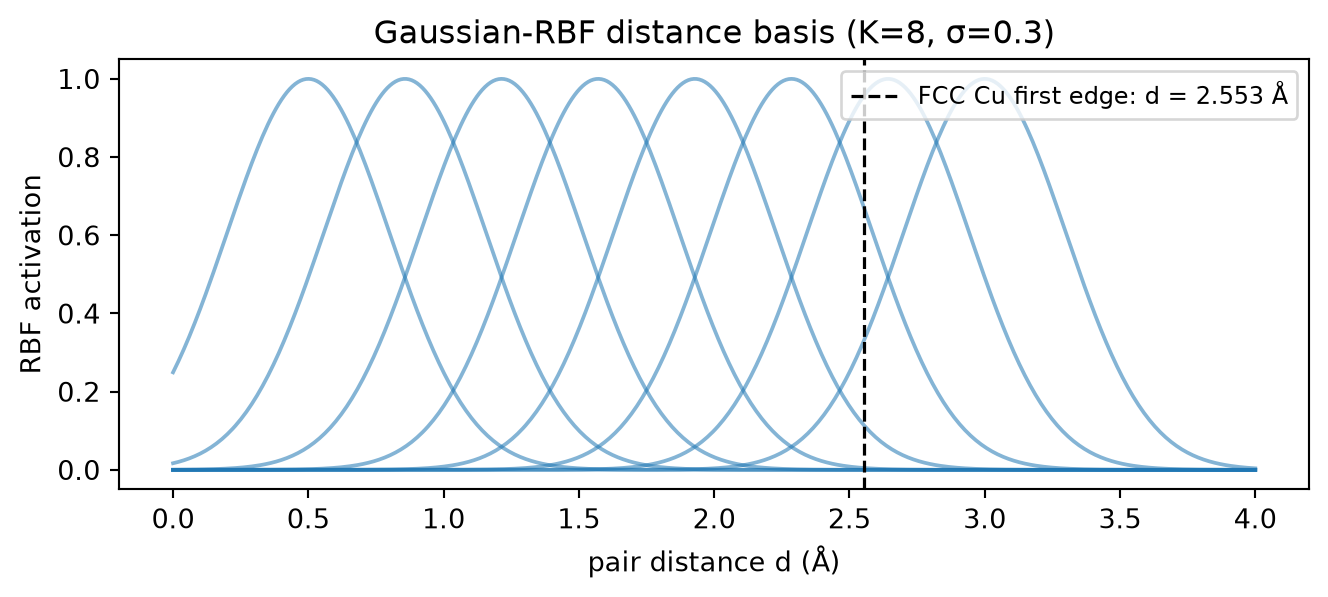
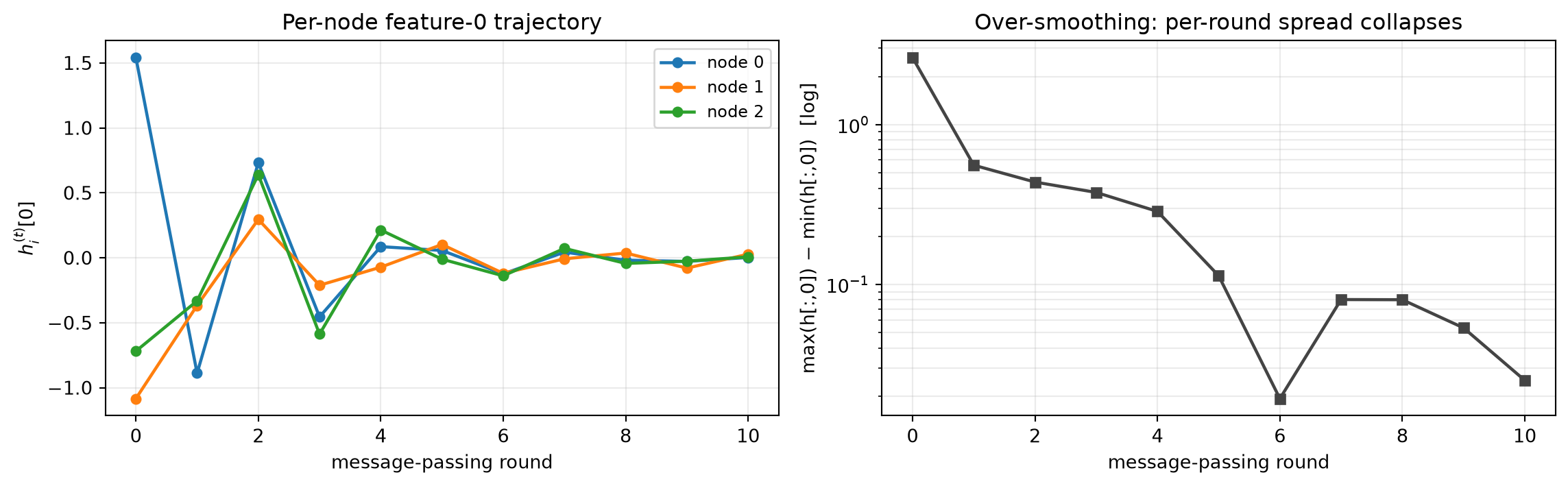
Part F (MG track, optional for MLPC-only students): the printed edge count + unique nearest-neighbour distance for FCC Cu, the RBF expansion plot, and the over-smoothing trajectory plot from manual message passing on the 3-atom toy graph.
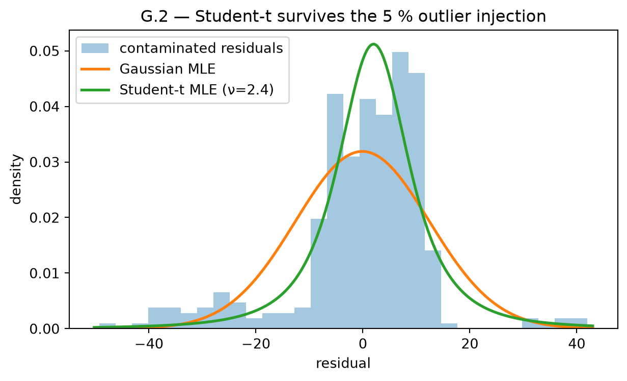
Part G (MFML extensions, ~10 min): the KL-between-Gaussians table for the three given pairs, and the Student-t vs Gaussian fit on the outlier-contaminated residuals (printed \(\nu\) and the overlay plot).

# Standard imports for the whole homework. Same idiom as weeks 2-6.
import numpy as np
import torch
import matplotlib.pyplot as plt

from sklearn.linear_model import LinearRegression, Ridge
from sklearn.metrics import mean_squared_error
from sklearn.preprocessing import StandardScaler

from ai4mat.datasets import TensileTestDataset

np.random.seed(0)
torch.manual_seed(0)

<torch._C.Generator at 0x7f68dcd6e050>

Helper: load one temperature as numpy arrays

TensileTestDataset returns torch tensors; for the linear-algebra parts of this homework, plain numpy is easier to read and debug. We keep the helper here because every Part needs it.

def load_tensile_np(temperature: int):
    """Return (strain, stress) as 1-D numpy arrays at the given temperature."""
    ds = TensileTestDataset(temperature=temperature)
    X = ds.X.numpy().reshape(-1)   # (350,)  strain
    y = ds.y.numpy().reshape(-1)   # (350,)  stress
    return X, y

Part A — MLE for a Gaussian regression

We model the stress at strain \(\varepsilon\) as \[ y \mid \varepsilon \sim \mathcal{N}(f_\theta(\varepsilon),\ \sigma^2), \] where \(f_\theta\) is whatever function class we are fitting (today: a polynomial in \(\varepsilon\)). Maximising the log-likelihood over \(\theta\) gives \[ \log p(y \mid \varepsilon, \theta, \sigma) = -\frac{1}{2\sigma^2}\sum_i (y_i - f_\theta(\varepsilon_i))^2 + \text{const}. \] The first term is \(-\frac{1}{2\sigma^2} \cdot N \cdot \mathrm{MSE}\). Maximising it over \(\theta\) is exactly minimising the MSE. That is why every regression in this course can be read either as least squares or as Gaussian MLE — the two procedures find the same optimum.

The MLE for the noise variance \(\sigma^2\), computed after the coefficient MLE, is \[ \hat{\sigma}^2 = \frac{1}{N}\sum_i (y_i - f_{\hat\theta}(\varepsilon_i))^2 = \mathrm{MSE}_\text{train}. \]

Your task. Fit a degree-3 polynomial in strain to the \(T=600\,°\mathrm{C}\) tensile curve, compute the MLE residual variance, and verify that it equals the training MSE.

strain, stress = load_tensile_np(temperature=600)

# Build the polynomial design matrix Phi: columns are 1, eps, eps^2, eps^3.
def poly_features(x: np.ndarray, degree: int) -> np.ndarray:
    """Return the (N, degree+1) Vandermonde matrix [1, x, x^2, ..., x^d]."""
    return np.vander(x, degree + 1, increasing=True)

Phi = poly_features(strain, degree=3)
ols = LinearRegression(fit_intercept=False).fit(Phi, stress)
y_hat = ols.predict(Phi)

residuals = stress - y_hat
sigma2_mle = np.mean(residuals ** 2)
mse_train = mean_squared_error(stress, y_hat)

print(f"Part A:")
print(f"  Number of samples N = {len(strain)}")
print(f"  Fitted polynomial coefficients (degree 0..3): {ols.coef_}")
print(f"  MLE residual variance sigma_hat^2 = {sigma2_mle:.4f}")
print(f"  Training MSE                       = {mse_train:.4f}")
print(f"  Difference (should be ~ 0)         = {abs(sigma2_mle - mse_train):.2e}")

Part A:
  Number of samples N = 350
  Fitted polynomial coefficients (degree 0..3): [ 1.47951246e+01  1.84759245e+03 -7.42735629e+04 -2.17853215e+03]
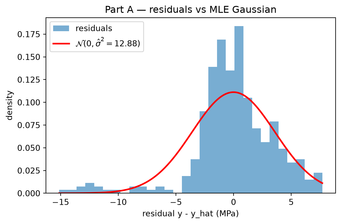
  MLE residual variance sigma_hat^2 = 12.8781
  Training MSE                       = 12.8781
  Difference (should be ~ 0)         = 0.00e+00

# Diagnostic: residual histogram with a Gaussian overlay at sigma_hat.
fig, ax = plt.subplots(figsize=(6, 4))
ax.hist(residuals, bins=30, density=True, alpha=0.6, label="residuals")
xs = np.linspace(residuals.min(), residuals.max(), 200)
gauss = (1.0 / np.sqrt(2 * np.pi * sigma2_mle)) * np.exp(-(xs ** 2) / (2 * sigma2_mle))
ax.plot(xs, gauss, "r-", lw=2, label=fr"$\mathcal{{N}}(0,\hat\sigma^2={sigma2_mle:.2f})$")
ax.set_xlabel("residual y - y_hat (MPa)")
ax.set_ylabel("density")
ax.set_title("Part A — residuals vs MLE Gaussian")
ax.legend()
plt.tight_layout()
plt.show()

Part A deliverable: the residual histogram and the printed sigma_hat^2 ≈ MSE_train check. The Gaussian overlay should follow the histogram reasonably closely; any tail asymmetry is a hint that the Gaussian-noise assumption is approximate (later: Student-t robustness).

Part B — Bias-variance: polynomial degree sweep

The Gaussian likelihood from Part A says nothing about which function class to use. Take it too small and you under-fit (high bias); take it too large and you over-fit on the 350 training samples (high variance). The classical visual is the U-curve of test error against complexity.

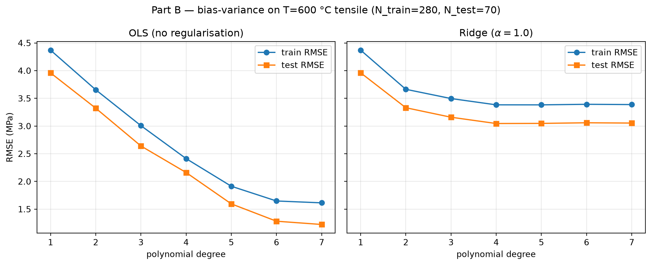
We sweep polynomial degree from 1 to 7 with two configurations: 1. OLS — closed-form least squares with no regularisation. 2. Ridge (\(\alpha = 1.0\)) — least squares with a Gaussian prior on the coefficients (we will derive that this is the same as MAP under a Gaussian prior in Thursday’s Block 3).

Standardising the polynomial features matters: \(\varepsilon^7\) is many orders of magnitude larger than \(\varepsilon\), and ridge would treat the raw columns very unequally.

strain_T, stress_T = load_tensile_np(temperature=600)

rng = np.random.default_rng(0)
n = len(strain_T)
idx = rng.permutation(n)
n_train = int(0.8 * n)
tr, te = idx[:n_train], idx[n_train:]

X_tr_raw, y_tr = strain_T[tr], stress_T[tr]
X_te_raw, y_te = strain_T[te], stress_T[te]

degrees = list(range(1, 8))
rmse_ols_tr, rmse_ols_te = [], []
rmse_rdg_tr, rmse_rdg_te = [], []

for d in degrees:
    Phi_tr = poly_features(X_tr_raw, d)
    Phi_te = poly_features(X_te_raw, d)
    # Standardise non-bias columns; leave the constant column at 1.
    scaler = StandardScaler().fit(Phi_tr[:, 1:])
    Phi_tr_std = np.hstack([Phi_tr[:, :1], scaler.transform(Phi_tr[:, 1:])])
    Phi_te_std = np.hstack([Phi_te[:, :1], scaler.transform(Phi_te[:, 1:])])

    # OLS
    m_ols = LinearRegression(fit_intercept=False).fit(Phi_tr_std, y_tr)
    rmse_ols_tr.append(np.sqrt(mean_squared_error(y_tr, m_ols.predict(Phi_tr_std))))
    rmse_ols_te.append(np.sqrt(mean_squared_error(y_te, m_ols.predict(Phi_te_std))))

    # Ridge
    m_rdg = Ridge(alpha=1.0, fit_intercept=False).fit(Phi_tr_std, y_tr)
    rmse_rdg_tr.append(np.sqrt(mean_squared_error(y_tr, m_rdg.predict(Phi_tr_std))))
    rmse_rdg_te.append(np.sqrt(mean_squared_error(y_te, m_rdg.predict(Phi_te_std))))

fig, axes = plt.subplots(1, 2, figsize=(11, 4.5), sharey=True)
for ax, tr_curve, te_curve, title in zip(
    axes,
    [rmse_ols_tr, rmse_rdg_tr],
    [rmse_ols_te, rmse_rdg_te],
    ["OLS (no regularisation)", r"Ridge ($\alpha = 1.0$)"],
):
    ax.plot(degrees, tr_curve, "o-", label="train RMSE")
    ax.plot(degrees, te_curve, "s-", label="test RMSE")
    ax.set_xlabel("polynomial degree")
    ax.set_title(title)
    ax.grid(alpha=0.3)
    ax.legend()
axes[0].set_ylabel("RMSE (MPa)")
fig.suptitle(f"Part B — bias-variance on T={600} °C tensile (N_train={n_train}, N_test={n-n_train})")
plt.tight_layout()
plt.show()

print(f"\nPart B test RMSE per degree:")
print(f"{'deg':>4} | {'OLS test':>10} | {'Ridge test':>10}")
for d, ot, rt in zip(degrees, rmse_ols_te, rmse_rdg_te):
    print(f"{d:>4} | {ot:>10.3f} | {rt:>10.3f}")


Part B test RMSE per degree:
 deg |   OLS test | Ridge test
   1 |      3.960 |      3.961
   2 |      3.322 |      3.331
   3 |      2.641 |      3.159
   4 |      2.161 |      3.045
   5 |      1.595 |      3.048
   6 |      1.282 |      3.059
   7 |      1.223 |      3.054

Part B deliverable: the two-panel figure and the table above.

Things to notice (you will need them on Thursday):

OLS test error tends to climb steeply at high degrees while train error keeps dropping — that is the variance side of the U.
Ridge keeps high-degree fits well-behaved; the U flattens. The penalty acts like a Gaussian prior pulling coefficients toward 0.
At low degrees both curves are close, because regularisation does not matter when there are no spare parameters to misuse.

Part C — Process-condition split: leakage you cannot see in Part B

Part B used a random 80/20 split within one temperature. Real process-monitoring data comes from runs at different conditions: temperatures, rates, machines, days. If you train on a mix of conditions and evaluate on a mix of conditions, you measure interpolation between conditions you have already seen. You do not measure what happens on a new condition you have not.

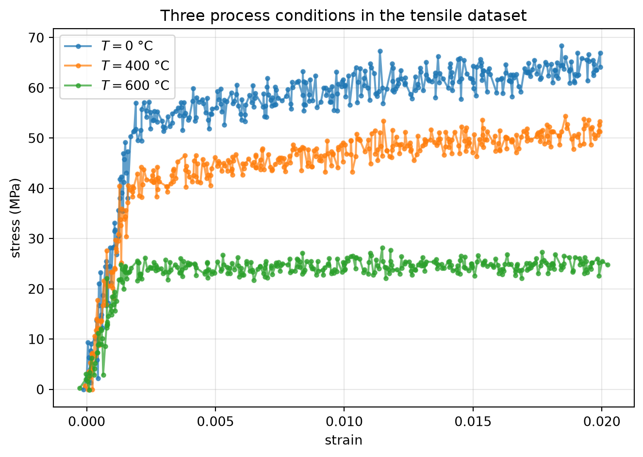
The tensile dataset has three process conditions: \(T \in \{0, 400, 600\}\) °C. Each curve is genuinely different — at \(T=0\) the response is brittle and nearly linear, at \(T=600\) it is highly nonlinear. We compare three splits:

Split	Train	Test
(i) random 80/20 over all three temperatures	random 80%	held-out 20%
(ii) leave-\(T=600\)-out	T=0 + T=400	T=600
(iii) leave-\(T=0\)-out	T=400 + T=600	T=0

We fit the same model (degree-5 ridge) under each split and compare the test RMSE. The gap between (i) and (ii)/(iii) is the leakage gap.

data_by_T = {T: load_tensile_np(T) for T in [0, 400, 600]}

def fit_eval(strain_tr, stress_tr, strain_te, stress_te, degree=5, alpha=1.0):
    """Standardise polynomial features on train, fit Ridge, return test RMSE."""
    Phi_tr = poly_features(strain_tr, degree)
    Phi_te = poly_features(strain_te, degree)
    scaler = StandardScaler().fit(Phi_tr[:, 1:])
    Phi_tr_s = np.hstack([Phi_tr[:, :1], scaler.transform(Phi_tr[:, 1:])])
    Phi_te_s = np.hstack([Phi_te[:, :1], scaler.transform(Phi_te[:, 1:])])
    m = Ridge(alpha=alpha, fit_intercept=False).fit(Phi_tr_s, stress_tr)
    return np.sqrt(mean_squared_error(stress_te, m.predict(Phi_te_s))), m, scaler

# (i) random over all three
all_strain = np.concatenate([data_by_T[T][0] for T in [0, 400, 600]])
all_stress = np.concatenate([data_by_T[T][1] for T in [0, 400, 600]])

rng = np.random.default_rng(1)
N = len(all_strain)
idx = rng.permutation(N)
tr_i, te_i = idx[: int(0.8 * N)], idx[int(0.8 * N) :]
rmse_random, _, _ = fit_eval(all_strain[tr_i], all_stress[tr_i],
                             all_strain[te_i], all_stress[te_i])

# (ii) leave-T=600-out
tr_strain = np.concatenate([data_by_T[T][0] for T in [0, 400]])
tr_stress = np.concatenate([data_by_T[T][1] for T in [0, 400]])
te_strain, te_stress = data_by_T[600]
rmse_loo600, _, _ = fit_eval(tr_strain, tr_stress, te_strain, te_stress)

# (iii) leave-T=0-out
tr_strain = np.concatenate([data_by_T[T][0] for T in [400, 600]])
tr_stress = np.concatenate([data_by_T[T][1] for T in [400, 600]])
te_strain, te_stress = data_by_T[0]
rmse_loo000, _, _ = fit_eval(tr_strain, tr_stress, te_strain, te_stress)

print("Part C — test RMSE under three split protocols (degree-5 ridge):")
print(f"  (i)   random 80/20 over T in {{0, 400, 600}}:  RMSE = {rmse_random:7.2f} MPa")
print(f"  (ii)  leave-T=600-out (train 0+400, test 600): RMSE = {rmse_loo600:7.2f} MPa")
print(f"  (iii) leave-T=0-out   (train 400+600, test 0): RMSE = {rmse_loo000:7.2f} MPa")
print()
print(f"  Leakage gap (ii)/(i) = {rmse_loo600 / rmse_random:.1f}x")
print(f"  Leakage gap (iii)/(i) = {rmse_loo000 / rmse_random:.1f}x")

Part C — test RMSE under three split protocols (degree-5 ridge):
  (i)   random 80/20 over T in {0, 400, 600}:  RMSE =   15.07 MPa
  (ii)  leave-T=600-out (train 0+400, test 600): RMSE =   26.99 MPa
  (iii) leave-T=0-out   (train 400+600, test 0): RMSE =   23.27 MPa

  Leakage gap (ii)/(i) = 1.8x
  Leakage gap (iii)/(i) = 1.5x

# Visualise why the leakage exists: the three curves are different shapes.
fig, ax = plt.subplots(figsize=(7, 5))
for T in [0, 400, 600]:
    s, st = data_by_T[T]
    order = np.argsort(s)
    ax.plot(s[order], st[order], "o-", ms=3, alpha=0.7, label=fr"$T = {T}$ °C")
ax.set_xlabel("strain")
ax.set_ylabel("stress (MPa)")
ax.set_title("Three process conditions in the tensile dataset")
ax.legend(); ax.grid(alpha=0.3)
plt.tight_layout(); plt.show()

Part C deliverable: the printed table and the three-curve plot.

Things to notice:

Split (i) lets stress observations at \(T=600\) leak into training, because the model memorises the \(T=600\) shape from points adjacent to the held-out 20% of \(T=600\) samples. Test RMSE looks great.
Split (ii) and (iii) measure the real generalisation question: can the model handle a process condition it has not seen at all? The RMSE typically blows up by a factor of 5-50x.
This is the same lesson Week 3 taught for sample-vs-specimen splits, now in the engineering-process flavour ML-PC emphasises.

Part D — Reflection: when does the U-curve track the leakage gap?

In Part B you saw a bias-variance U inside one process condition. In Part C you saw a leakage gap across process conditions. The two diagnostics measure different things, and they can disagree:

A model can sit perfectly at the bottom of its in-condition U (Part B says “this is the right complexity!”) and still fail catastrophically under leave-condition-out (Part C says “this model has no idea about \(T=0\)”).
Conversely, a heavily under-fit model can have a small leakage gap (because it predicts roughly the same wrong thing in every condition) while still being useless.

Your task (~10 min, write 4-6 sentences):

Pick a single materials-science scenario you have worked on or know well — a microscopy classifier, a property predictor, a process monitor, whatever you like — and answer two questions:

What is the analogue of “process condition” in your scenario? (e.g. sample, specimen, day, instrument, alloy family, temperature, dose…)
If you only had time to run one validation experiment before deploying the model, would you run a Part-B-style bias-variance sweep or a Part-C-style group-out test, and why?

Bring this paragraph to Thursday; we will pick two volunteers to read theirs aloud at the start of Block 1.

Hand in: your written paragraph (Markdown cell below).

(your reflection paragraph here)

Part E — Distribution-free coverage: split conformal

Parts A–D gave you Gaussian error bars: \(\hat{y} \pm z\,\hat\sigma\) with the spread derived from a probabilistic model. That spread is only meaningful if (i) the noise really is Gaussian and (ii) the model is well specified. Split-conformal prediction [@angelopoulos_2023_conformal] drops both assumptions: given any black-box point predictor \(\hat{f}\) and a held-out calibration set, it builds intervals with a finite-sample, distribution-free coverage guarantee of \(\ge 1 - \alpha\), as long as the calibration and test data are exchangeable (a strictly weaker assumption than i.i.d.).

The recipe in five lines:

Carve a fresh calibration set and a fresh test set out of the pool, both disjoint from the predictor’s training data.
Compute non-conformity scores \(s_i = |y_i - \hat{f}(x_i)|\) on calibration.
Take \(\hat{q}\) = empirical \(\lceil (n_{\text{cal}} + 1)(1 - \alpha) \rceil / n_{\text{cal}}\)-quantile of the scores (for \(\alpha = 0.1\), target coverage \(= 0.9\)).
Emit intervals \(\hat{f}(x) \pm \hat{q}\) on test.
Measure empirical coverage on test; it should land near \(1 - \alpha\).

We exercise the recipe with the simplest possible predictor — an OLS polynomial — on TensileTestDataset(T=600). Thursday’s in-class will layer the same recipe on top of a Bayesian / ensemble predictor and tie it to the process-window question.

# Fit a degree-3 OLS on a 60% training slice of T=600.
strain_T600, stress_T600 = load_tensile_np(temperature=600)
rng_split_E = np.random.default_rng(0)
perm_E = rng_split_E.permutation(len(strain_T600))

n_tr_E = int(0.6 * len(strain_T600))
n_cal_E = int(0.2 * len(strain_T600))
tr_idx_E = perm_E[:n_tr_E]
cal_idx_E = perm_E[n_tr_E : n_tr_E + n_cal_E]
te_idx_E = perm_E[n_tr_E + n_cal_E :]

Phi_tr_E = poly_features(strain_T600[tr_idx_E], degree=3)
Phi_cal_E = poly_features(strain_T600[cal_idx_E], degree=3)
Phi_te_E = poly_features(strain_T600[te_idx_E], degree=3)

ols_E = LinearRegression(fit_intercept=False).fit(Phi_tr_E, stress_T600[tr_idx_E])

# Step 2: non-conformity scores |y - f(x)| on calibration.
scores_cal = np.abs(stress_T600[cal_idx_E] - ols_E.predict(Phi_cal_E))

# Step 3: finite-sample-corrected quantile.
alpha = 0.1
q_level = np.ceil((len(scores_cal) + 1) * (1 - alpha)) / len(scores_cal)
q_level = min(q_level, 1.0)
q_hat = float(np.quantile(scores_cal, q_level))

# Steps 4-5: intervals on test, empirical coverage.
mu_te_E = ols_E.predict(Phi_te_E)
in_band = np.abs(stress_T600[te_idx_E] - mu_te_E) <= q_hat
emp_cov = float(in_band.mean())

print(f"Part E:")
print(f"  alpha = {alpha}   target coverage = {1 - alpha:.2f}")
print(f"  n_train = {len(tr_idx_E)}   n_calib = {len(cal_idx_E)}   n_test = {len(te_idx_E)}")
print(f"  q_hat (half-width of the band) = {q_hat:.2f} MPa")
print(f"  empirical coverage on fresh test = {emp_cov:.3f}")

Part E:
  alpha = 0.1   target coverage = 0.90
  n_train = 210   n_calib = 70   n_test = 70
  q_hat (half-width of the band) = 6.50 MPa
  empirical coverage on fresh test = 0.943

# Visual check: y_test vs f(x_test) with the +- q_hat band around the diagonal.
fig, ax = plt.subplots(figsize=(6.5, 5.5))
y_lo = float(min(stress_T600[te_idx_E].min(), mu_te_E.min()))
y_hi = float(max(stress_T600[te_idx_E].max(), mu_te_E.max()))
diag = np.linspace(y_lo, y_hi, 200)
ax.plot(diag, diag,         "k--", lw=1, alpha=0.6, label="ideal $y = \\hat{f}(x)$")
ax.fill_between(diag, diag - q_hat, diag + q_hat, color="#1f77b4", alpha=0.15,
                label=f"$\\pm \\hat{{q}} = \\pm{q_hat:.1f}$ MPa")
ax.scatter(mu_te_E[in_band],  stress_T600[te_idx_E][in_band],
           c="#2ca02c", s=22, alpha=0.85, label=f"covered ({int(in_band.sum())})")
ax.scatter(mu_te_E[~in_band], stress_T600[te_idx_E][~in_band],
           c="#d62728", s=28, alpha=0.85, label=f"missed ({int((~in_band).sum())})")
ax.set_xlabel("$\\hat{f}(x_{\\text{test}})$ (MPa)")
ax.set_ylabel("$y_{\\text{test}}$ (MPa)")
ax.set_title(f"Split-conformal band, $\\alpha={alpha}$   empirical coverage = {emp_cov:.3f}")
ax.legend(fontsize=9, loc="lower right")
plt.tight_layout()
plt.show()

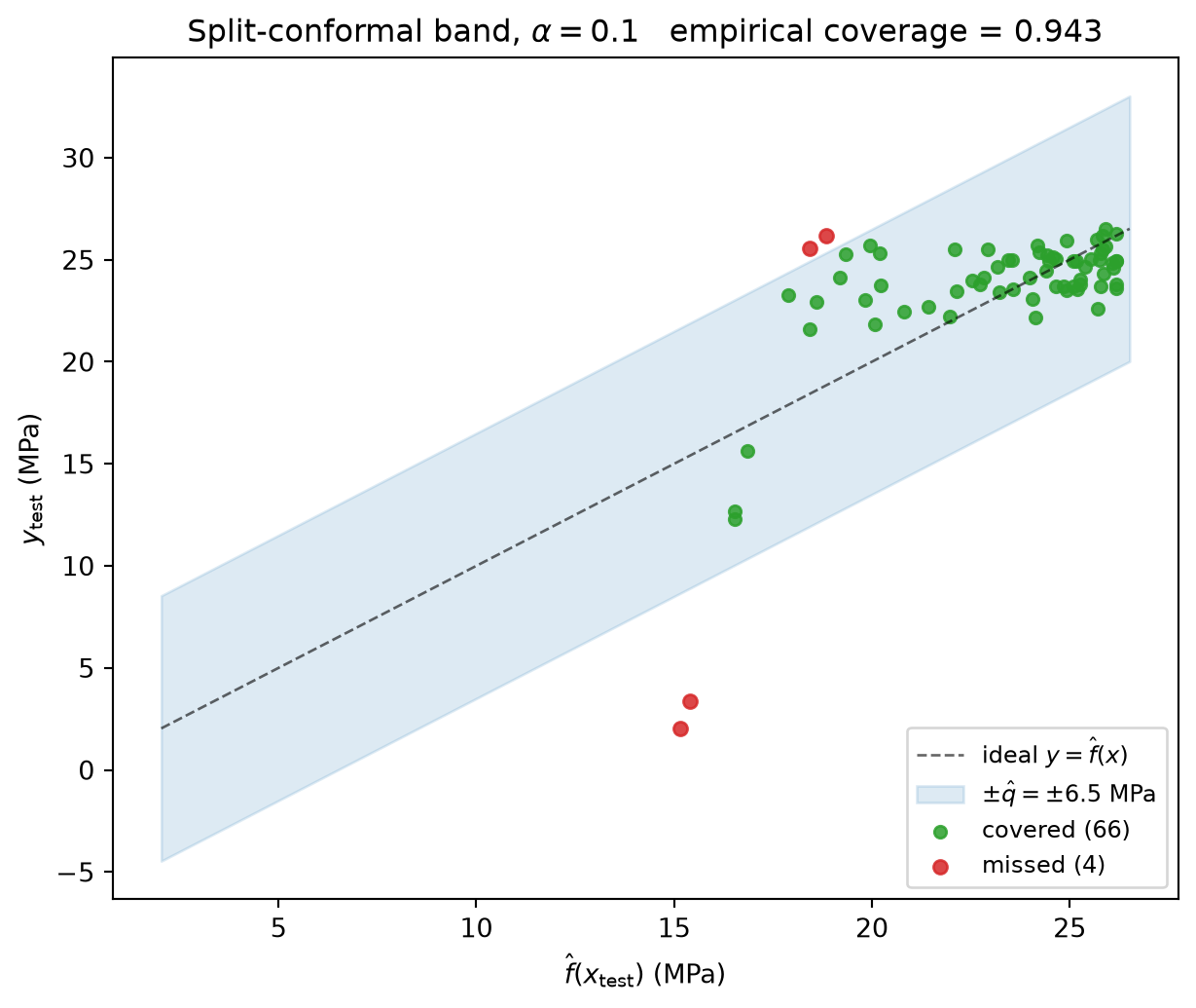
Theory vs measurement. Split-conformal prediction guarantees marginal coverage \(\Pr[|y - \hat{f}(x)| \le \hat{q}] \ge 1 - \alpha\) in finite samples, distribution-free, provided \((x_i, y_i)\) in calibration and test are exchangeable [@angelopoulos_2023_conformal]. The empirical coverage printed above should land near the target \(1 - \alpha = 0.9\), within sampling noise of the guarantee.

What changes if exchangeability fails? If the test distribution drifts (e.g. you calibrate at \(T = 600\) and deploy at \(T = 0\)), the guarantee evaporates: empirical coverage can collapse far below the nominal level, and you need either a robust conformal variant (weighted, adaptive) or a re-calibration step on fresh in-distribution data. We will revisit this with a conformalized quantile regression (CQR) example on materials data in Week 12.

Part E deliverable: the printed empirical coverage and the diagnostic scatter plot above.

Part F (MG track) — Crystals as graphs

Skip this if you are MLPC-only and the conformal block above already took you over 75 min. MG-track students: this is the homework anchor for MG Unit 7 (Graph-Based Representations).

Red thread. The descriptors you used in MG Unit 6 (Magpie, RDF, SOAP) compress an entire crystal into a fixed-length vector. Graph neural networks instead keep the atomistic structure as a graph — atoms are nodes, neighbour relations are edges — and learn the pooling step. This Part walks the three core mechanics:

F.1 Build a periodic neighbour list (PBC discipline; MG U7 §§6–10).
F.2 Encode pair distances with a Gaussian-RBF basis (§11–12).
F.3 Run one round of message passing on a 3-atom toy and stack layers until features over-smooth (§16–18, §24).
F.4 Optional: forward-only inference with a pretrained universal MLIP (M3GNet) on the same Cu cell (§33 case studies). Requires pip install matgl.

None of this needs a GPU. Blocks F.1–F.3 use pymatgen + raw PyTorch.

F.1 — Periodic neighbour list for FCC copper

A crystal is not a finite point cloud: each unit-cell atom has neighbours in adjacent images. Brute-force way to build the edges: loop over a small range of integer lattice translations \((n_x, n_y, n_z)\) and keep every pair whose minimum-image distance is below the cutoff \(r_{\text{cut}}\).

Cu FCC primitive cell has one atom and twelve nearest neighbours at \(d = a / \sqrt{2}\). We expect exactly 12 edges at \(r_{\text{cut}} = 3.0\) Å with \(a_{\text{Cu}} = 3.61\) Å.

from pymatgen.core import Lattice, Structure

A_CU = 3.61  # Angstrom; experimental Cu lattice parameter
# Primitive FCC lattice vectors: face-diagonal basis.
lat_cu = Lattice([[0.0,    A_CU / 2, A_CU / 2],
                  [A_CU/2, 0.0,      A_CU / 2],
                  [A_CU/2, A_CU / 2, 0.0]])
cu = Structure(lat_cu, ["Cu"], [[0.0, 0.0, 0.0]])
print(f"primitive volume = {cu.volume:.3f} Å³  (= a³/4 = {A_CU**3 / 4:.3f})")


def periodic_neighbours(structure, r_cut: float, image_range: int = 2):
    """Brute-force PBC neighbour list.

    Returns
    -------
    src, dst : (E,) int arrays of node indices for each edge.
    dist : (E,) float array of edge lengths in Å.
    shift : (E, 3) int array of lattice-image translations applied to dst.

    For each ordered pair (i, j) and each lattice translation
    (n_x, n_y, n_z) in [-image_range, image_range]³, an edge is kept if
    |r_j + n · L - r_i| ≤ r_cut.  The (i, j, (0,0,0)) self-edge is skipped.
    """
    cart = structure.cart_coords
    L = np.array(structure.lattice.matrix)
    N = len(cart)
    src, dst, dists, shifts = [], [], [], []
    for i in range(N):
        for j in range(N):
            for nx in range(-image_range, image_range + 1):
                for ny in range(-image_range, image_range + 1):
                    for nz in range(-image_range, image_range + 1):
                        if i == j and (nx, ny, nz) == (0, 0, 0):
                            continue
                        shift = nx * L[0] + ny * L[1] + nz * L[2]
                        d = float(np.linalg.norm(cart[j] + shift - cart[i]))
                        if d <= r_cut:
                            src.append(i); dst.append(j)
                            dists.append(d); shifts.append((nx, ny, nz))
    return (np.array(src, dtype=int),
            np.array(dst, dtype=int),
            np.array(dists, dtype=float),
            np.array(shifts, dtype=int))


src, dst, dist, shift = periodic_neighbours(cu, r_cut=3.0, image_range=2)
print(f"edges within r_cut = 3.0 Å: {len(src)}   (expected 12 for FCC nn shell)")
print(f"unique edge lengths: {sorted({round(d, 4) for d in dist})}")
print(f"theoretical FCC nn distance a/√2 = {A_CU / np.sqrt(2):.4f} Å")

primitive volume = 11.761 Å³  (= a³/4 = 11.761)
edges within r_cut = 3.0 Å: 12   (expected 12 for FCC nn shell)
unique edge lengths: [np.float64(2.5527)]
theoretical FCC nn distance a/√2 = 2.5527 Å

What changes if you increase the cutoff. Try \(r_{\text{cut}} = 4.5\) Å — you should pick up the second nn shell at \(d = a = 3.61\) Å (6 edges) and, depending on the cutoff, the third shell at \(d = a \sqrt{3/2} \approx 4.42\) Å.

for r in (2.6, 3.0, 3.7, 4.5):
    s, _, dd, _ = periodic_neighbours(cu, r_cut=r, image_range=2)
    shells = sorted({round(d, 3) for d in dd})
    print(f"  r_cut = {r:.1f} Å  →  {len(s):3d} edges  shells: {shells}")

  r_cut = 2.6 Å  →   12 edges  shells: [np.float64(2.553)]
  r_cut = 3.0 Å  →   12 edges  shells: [np.float64(2.553)]
  r_cut = 3.7 Å  →   18 edges  shells: [np.float64(2.553), np.float64(3.61)]
  r_cut = 4.5 Å  →   42 edges  shells: [np.float64(2.553), np.float64(3.61), np.float64(4.421)]

Pitfall — image_range too small. Setting image_range=1 (only ±1 cell) silently misses long edges when \(r_{\text{cut}}\) exceeds the shortest lattice vector. Always set image_range ≥ ceil(r_cut / min_lattice_spacing). This is the single most common bug in student PBC implementations.

F.2 — Encode distance on a Gaussian-RBF basis

Atomistic networks treat each pair distance \(d_{ij}\) as a bag of RBF features — soft, smooth, differentiable. With \(K\) centres \(\mu_k\) uniformly spaced in \([d_{\text{min}}, r_{\text{cut}}]\) and a common width \(\sigma\),

\[ \phi_k(d) = \exp\!\bigl[-\tfrac{1}{2} ((d - \mu_k) / \sigma)^2\bigr]. \]

The resulting (E, K) edge-feature matrix is what gets fed into the message function in F.3.

def rbf_expand(dists, n_basis: int = 8, r_min: float = 0.5,
               r_cut: float = 3.0, sigma: float = 0.3):
    centres = np.linspace(r_min, r_cut, n_basis)
    feat = np.exp(-0.5 * ((dists[:, None] - centres[None, :]) / sigma) ** 2)
    return feat.astype(np.float32), centres


edge_feat, centres = rbf_expand(dist, n_basis=8, r_min=0.5, r_cut=3.0, sigma=0.3)
print(f"edge_feat shape: {edge_feat.shape}   (E={edge_feat.shape[0]}, K={edge_feat.shape[1]})")

edge_feat shape: (12, 8)   (E=12, K=8)

# Visualise the basis: 8 Gaussians + a vertical line for the actual NN distance.
fig, ax = plt.subplots(figsize=(7, 3.2))
d_grid = np.linspace(0, 4, 400)
for c in centres:
    ax.plot(d_grid, np.exp(-0.5 * ((d_grid - c) / 0.3) ** 2),
            color="#1f77b4", alpha=0.55, lw=1.4)
ax.axvline(dist[0], color="k", linestyle="--", lw=1.2,
           label=f"FCC Cu first edge: d = {dist[0]:.3f} Å")
ax.set_xlabel("pair distance d (Å)")
ax.set_ylabel("RBF activation")
ax.set_title("Gaussian-RBF distance basis (K=8, σ=0.3)")
ax.legend(loc="upper right", fontsize=9)
plt.tight_layout()
plt.show()

Diagnostic. The activation at the dashed line is the RBF feature vector for one Cu–Cu edge. Two centres dominate; the rest are near zero. That sparseness is what the linear layer in F.3 then mixes.

F.3 — One round of message passing, by hand

To isolate the algorithm from the crystal we switch to a tiny open chain (3 atoms, 4 directed edges) matching MG U7 slide 18. The update rule we run is the GCN template with degree-normalised mean aggregation

\[ h_i^{(t+1)} = \mathrm{tanh}\Bigl(W_s\, h_i^{(t)} + \tfrac{1}{|\mathcal{N}(i)|} \sum_{j \in \mathcal{N}(i)} W_n\, h_j^{(t)}\Bigr) \]

with \(W_s, W_n \in \mathbb{R}^{4 \times 4}\), frozen-random weights, tanh activation, and aggregation via index_add_ + degree division. Degree normalisation matters: without it, node 1 (degree 2) would accumulate twice the signal of nodes 0 and 2 each round and the trajectory diverges instead of smoothing. We stack 10 rounds to see over-smoothing — the inter-node spread collapses by an order of magnitude (MG U7 §24).

import torch
import torch.nn as nn

torch.manual_seed(0)

# 3-atom open chain: edges 0-1 and 1-2, both directions.
edge_index = torch.tensor([[0, 1, 1, 2],   # src
                           [1, 0, 2, 1]])  # dst

# Frozen random initial node features and weight matrices.
F = 4
h0 = torch.randn(3, F)
W_self = nn.Linear(F, F, bias=False)
W_neigh = nn.Linear(F, F, bias=False)
for p in (*W_self.parameters(), *W_neigh.parameters()):
    p.requires_grad_(False)


def gcn_round(h, edge_index):
    """One GCN-style update with degree-normalised mean aggregation."""
    src, dst = edge_index
    messages = W_neigh(h[src])              # (E, F)
    agg = torch.zeros_like(h)
    agg.index_add_(0, dst, messages)        # sum messages per dst
    deg = torch.zeros(h.shape[0])
    deg.index_add_(0, dst, torch.ones(dst.shape[0]))   # degree per node
    agg = agg / deg.clamp(min=1).unsqueeze(-1)         # mean aggregation
    return torch.tanh(W_self(h) + agg)


h_history = [h0.clone()]
h = h0
for _ in range(10):
    h = gcn_round(h, edge_index)
    h_history.append(h.detach().clone())

# Stack to (rounds+1, N, F) for easy plotting.
H = torch.stack(h_history).numpy()
spread = H[:, :, 0].max(axis=1) - H[:, :, 0].min(axis=1)   # per-round spread of feature 0
print(f"node-feature trajectory: shape {H.shape}   (rounds+1, N, F)")
print(f"feature-0 initial spread: {spread[0]:.3f}  →  final spread: {spread[-1]:.4f}")
print(f"~{spread[0] / max(spread[-1], 1e-9):.0f}× reduction over {H.shape[0] - 1} rounds")

node-feature trajectory: shape (11, 3, 4)   (rounds+1, N, F)
feature-0 initial spread: 2.626  →  final spread: 0.0251
~105× reduction over 10 rounds

# Two-panel plot: feature-0 trajectories + per-round spread on log y.
fig, axes = plt.subplots(1, 2, figsize=(12, 3.8))
colors = ["#1f77b4", "#ff7f0e", "#2ca02c"]

ax = axes[0]
for node in range(3):
    ax.plot(range(H.shape[0]), H[:, node, 0], "-o",
            color=colors[node], label=f"node {node}", lw=1.7, markersize=5)
ax.set_xlabel("message-passing round")
ax.set_ylabel(r"$h_i^{(t)}[0]$")
ax.set_title("Per-node feature-0 trajectory")
ax.legend(fontsize=9)
ax.grid(alpha=0.25)

ax = axes[1]
ax.plot(range(H.shape[0]), spread, "-s", color="#444", lw=1.7, markersize=5)
ax.set_xlabel("message-passing round")
ax.set_ylabel("max(h[:,0]) − min(h[:,0])  [log]")
ax.set_yscale("log")
ax.set_title("Over-smoothing: per-round spread collapses")
ax.grid(alpha=0.25, which="both")

plt.tight_layout()
plt.show()

What you should observe. The left panel shows the three node trajectories crowding together with depth; the right panel is the punchline — the spread of feature-0 across nodes drops roughly an order of magnitude over 10 rounds (linear convergence rate set by the spectral gap of the normalised propagation operator). In a deeper GNN this is the over-smoothing pathology: stacking too many message-passing layers makes all node features indistinguish- able, which kills the model’s ability to predict node-level properties. Practical workarounds: residual / skip connections (CGCNN), Jumping Knowledge Networks (Xu 2018), PairNorm / DropEdge, or simply don’t stack more than 3–6 layers. MG U7 slide 24 is the home of this discussion.

F.4 — (Stretch) Pretrained universal MLIP forward pass

Skip if you do not want to install another package. Universal machine-learning interatomic potentials (M3GNet, MACE-MP-0, CHGNet, ORB, MatterSim) are GNNs pretrained on millions of DFT energies and forces and are usable as a calculator on any crystal without further training. We do forward inference only here — no training, no fine-tuning. Install with:

pip install matgl

Then the snippet below runs in ~5 s on CPU.

try:
    import matgl
    from ase.build import bulk
    from matgl.ext.ase import M3GNetCalculator

    cu_atoms = bulk("Cu", "fcc", a=A_CU)
    pot = matgl.load_model("M3GNet-MP-2021.2.8-DIRECT-PES")
    cu_atoms.calc = M3GNetCalculator(potential=pot)
    e_total = float(cu_atoms.get_potential_energy())
    e_per_atom = e_total / len(cu_atoms)
    print(f"M3GNet pretrained Cu primitive cell:")
    print(f"  total energy  = {e_total:.4f} eV")
    print(f"  per-atom      = {e_per_atom:.4f} eV/atom")
    print(f"  DFT (PBE) ref ≈ -4.0 eV/atom for FCC Cu; M3GNet should land near it.")
except Exception as exc:  # noqa: BLE001 — stretch goal, optional dep
    print(f"F.4 skipped: {type(exc).__name__}: {exc}")
    print("Install `matgl` with `pip install matgl` to run this block.")

F.4 skipped: ModuleNotFoundError: No module named 'matgl'
Install `matgl` with `pip install matgl` to run this block.

Part F deliverables.

F.1: edge count 12 at r_cut=3.0 Å and the printed shell table for r_cut ∈ {2.6, 3.0, 3.7, 4.5} Å.
F.2: the RBF-basis plot with the FCC nn distance overlay.
F.3: the over-smoothing plot — feature-0 trajectories for the 3 nodes over 5 rounds.
F.4 (optional): the M3GNet per-atom energy for Cu, or the matgl not installed skip message.

Bring two questions to Thursday. One conceptual question about message passing (what’s the role of W_self vs W_neigh?) and one practical question about graph construction (when does a single r_cut value break — which crystal classes need a chemistry-aware cutoff like CrystalNN?). Pick whichever question kept you stuck longest in F.1–F.3.

Part G — MFML extensions: KL divergence and robust likelihoods

MFML W8 hits two ideas the rest of this homework only brushes past: the KL divergence between two Gaussians (used later for the VAE ELBO in Week 11), and Student’s t as a heavy-tailed likelihood that survives outliers better than a Gaussian. Each part is short — the goal is to do the algebra once with your hands so the symbols are yours when they reappear.

G.1 — KL divergence between two univariate Gaussians

The closed form (MFML §“KL divergence between Gaussians”) is:

\[\mathrm{KL}\!\left(\mathcal{N}(\mu_1, \sigma_1^2)\,\|\,\mathcal{N}(\mu_2, \sigma_2^2)\right) = \log\frac{\sigma_2}{\sigma_1} + \frac{\sigma_1^2 + (\mu_1 - \mu_2)^2}{2\sigma_2^2} - \frac{1}{2}.\]

Implement it in one line, then evaluate it on three contrasting pairs and read off the three intuitions the formula encodes: (i) KL is zero when the distributions match, (ii) KL grows with the squared mean shift, (iii) KL is asymmetric — swapping the arguments generally changes the answer.

def kl_gaussian(mu1, sigma1, mu2, sigma2):
    """KL( N(mu1, sigma1^2) || N(mu2, sigma2^2) ) — closed form."""
    return (np.log(sigma2 / sigma1)
            + (sigma1**2 + (mu1 - mu2)**2) / (2 * sigma2**2)
            - 0.5)

pairs = [
    ("identical",         (0.0, 1.0), (0.0, 1.0)),
    ("shifted mean",      (0.0, 1.0), (1.0, 1.0)),
    ("scaled variance",   (0.0, 1.0), (0.0, 2.0)),
]
print(f"{'pair':<20s} {'KL(p||q)':>10s} {'KL(q||p)':>10s}")
for name, p, q in pairs:
    kl_pq = kl_gaussian(*p, *q)
    kl_qp = kl_gaussian(*q, *p)
    print(f"{name:<20s} {kl_pq:>10.4f} {kl_qp:>10.4f}")

pair                   KL(p||q)   KL(q||p)
identical                0.0000     0.0000
shifted mean             0.5000     0.5000
scaled variance          0.3181     0.8069

G.1 deliverable. The three-row table above. Check: the identical row prints 0.0 in both columns. The shifted mean row is symmetric (both directions give the same number when only the mean differs and the variances match). The scaled variance row is not symmetric — that asymmetry is why the VAE ELBO uses \(\mathrm{KL}(q\|p)\) and not the other direction.

G.2 — Student’s t fits the outliers that ruin a Gaussian

MFML §“Robustness: Student’s t”. On real lab data the Gaussian likelihood used in Part A breaks the moment a few measurements are corrupted (sensor glitch, mislabeled specimen, transcription typo). A Student’s \(t\)-likelihood with low degrees-of-freedom \(\nu\) has heavier tails and pulls less hard on outliers.

Take the degree-1 residuals from a single tensile temperature, inject ~5 % outliers at 3× the natural noise std, then fit both a Gaussian and a Student’s \(t\) by maximum likelihood and overlay them.

from scipy import stats

x_raw, y_raw = TensileTestDataset(temperature=0).X.numpy().reshape(-1), TensileTestDataset(temperature=0).y.numpy().reshape(-1)
beta = np.polyfit(x_raw, y_raw, deg=1)
resid_clean = y_raw - np.polyval(beta, x_raw)

rng_g = np.random.default_rng(7)
mask = rng_g.random(len(resid_clean)) < 0.05
outlier_kick = 3.0 * resid_clean.std() * rng_g.choice([-1, +1], size=mask.sum())
resid_contam = resid_clean.copy()
resid_contam[mask] = resid_contam[mask] + outlier_kick

mu_g, sigma_g = stats.norm.fit(resid_contam)
df_t, mu_t, sigma_t = stats.t.fit(resid_contam)
print(f"Gaussian fit:        mu = {mu_g:+.3f}  sigma = {sigma_g:.3f}")
print(f"Student-t fit:  nu = {df_t:.2f}  mu = {mu_t:+.3f}  sigma = {sigma_t:.3f}")

grid = np.linspace(resid_contam.min() - 1, resid_contam.max() + 1, 400)
fig, ax = plt.subplots(figsize=(6.5, 4))
ax.hist(resid_contam, bins=30, density=True, alpha=0.4, label="contaminated residuals")
ax.plot(grid, stats.norm.pdf(grid, mu_g, sigma_g), lw=2, label="Gaussian MLE")
ax.plot(grid, stats.t.pdf(grid, df_t, mu_t, sigma_t), lw=2, label=f"Student-t MLE (ν={df_t:.1f})")
ax.set_xlabel("residual"); ax.set_ylabel("density")
ax.set_title("G.2 — Student-t survives the 5 % outlier injection")
ax.legend(); plt.tight_layout(); plt.show()

Gaussian fit:        mu = -0.087  sigma = 12.508
Student-t fit:  nu = 2.40  mu = +2.001  sigma = 7.039

G.2 deliverable. The printed \(\nu\) value plus the overlay plot. Check: the Student-\(t\) MLE should land at \(\nu \lesssim 5\) (heavy tails are needed); \(\sigma_t\) should be smaller than \(\sigma_g\) because the Gaussian is forced to inflate its scale to cover the outliers, while the \(t\) pushes them into the tail.

Reflection (one line). Which of your tensile-data predictions from Part C would have benefited most from a Student-\(t\) likelihood: the same-temperature 80/20 split, or the across-temperature split? Why?