Week 9 — Homework (do BEFORE the Thursday exercise)
This notebook is the mandatory warm-up for the Week 9 in-class exercise. Thursday braids three lectures, and this homework primes all three legs:
MFML Unit 9 — latent spaces & representation learning. You put the three projection lenses in your hands here: linear (PCA), nonlinear-visual (t-SNE/UMAP), and learned-without-labels (contrastive augmentation).
ML-PC Unit 9 — those same tools applied to characterisation signals (spectra). Thursday only; nothing to pre-build.
MG Unit 8 — Regression and generalization in materials data: split design, chemistry-family leakage, the mandatory baseline ladder, per-region residual diagnostics, and the seven-point trustworthy-reporting checklist. (This is not the SchNet/CGCNN/MEGNet architecture lecture — that is MG Unit 9, next week.) Part E below is the scaffolded prep for this leg.
Time: ~90 minutes.
Red thread
Parts A–D: a learned coordinate system — set by PCA, t-SNE, an autoencoder, or a contrastive loss — only earns trust once we ask what does the geometry organise by, and how do we measure that quantitatively? Part E flips to the orthogonal MG question: once you have a materials regressor, how do you know its number is scientifically trustworthy? In materials, the answer is not a tighter loss — it is split design, residual analysis, and reporting discipline. You build the projection tools on a clean image dataset (Ising); you warm up the regression-trust toolkit on the real MatBenchDataset perovskites benchmark. Thursday integrates both on spectra and on crystal data.
What this homework is
Part
Min
Topic
Lecture anchor
A
20
Hand-rolled PCA on Ising-full; reconstruction error vs latent dim
MFML §“PCA as a linear AE”, §“Reconstruction error vs latent dim”
B
25
t-SNE and UMAP on Ising-full latents; distance trap; n_neighbors sweep
MFML §“t-SNE”, §“UMAP — the 2026 default” [@mcinnes_2018_umap]
C
12
Augmentation pipeline for contrastive learning — no training; data-prep only
MFML §“Positive pair construction”, §“Augmentations as the prior”
D
8
Reflection: when does each method help?
bridge to Thursday Blocks 3 & 6
E
25
MG U8 prep: leakage-safe splits, baseline-ladder warm-up, a residual table, the checklist
What you must hand in (or be able to show on Thursday)
Part A: reconstruction-error-vs-k curve for k ∈ {1, 2, 4, 8, 16, 32} on Ising-full; printed table of MSE values.
Part B: 2-D t-SNE plot of the Ising bottleneck features, with the “distance trap” pair annotated; pixel-vs-tSNE distance comparison; 2×2 grid of UMAP layouts at n_neighbors ∈ {5, 15, 50, 200} with runtimes; one-sentence verdict on which method preserves global structure better.
Part C: pairwise pixel-distance histograms showing your make_positive_pair breaks pixel similarity while preserving class.
Part D: paragraph (~5 sentences) on PCA vs t-SNE vs contrastive.
Part E: (i) the random / CV / family MAE table with the \(\Delta_\text{shift}\) gap filled in; (ii) your one-line answer to “which split matches a new-chemistry discovery claim?”; (iii) the per-family residual table; (iv) your filled-in 7-point checklist score for the MatBench regressor.
# Standard imports for the whole homework. Same idiom as weeks 2-6.import numpy as npimport torchimport torch.nn.functional as Fimport matplotlib.pyplot as pltfrom sklearn.decomposition import PCA as SklearnPCAfrom sklearn.manifold import TSNEfrom sklearn.linear_model import Ridgefrom sklearn.ensemble import GradientBoostingRegressorfrom sklearn.metrics import mean_absolute_errorfrom ai4mat.datasets import IsingDatasetnp.random.seed(0)torch.manual_seed(0)
<torch._C.Generator at 0x7f5cf5d122f0>
Part A — Hand-rolled PCA on Ising-full
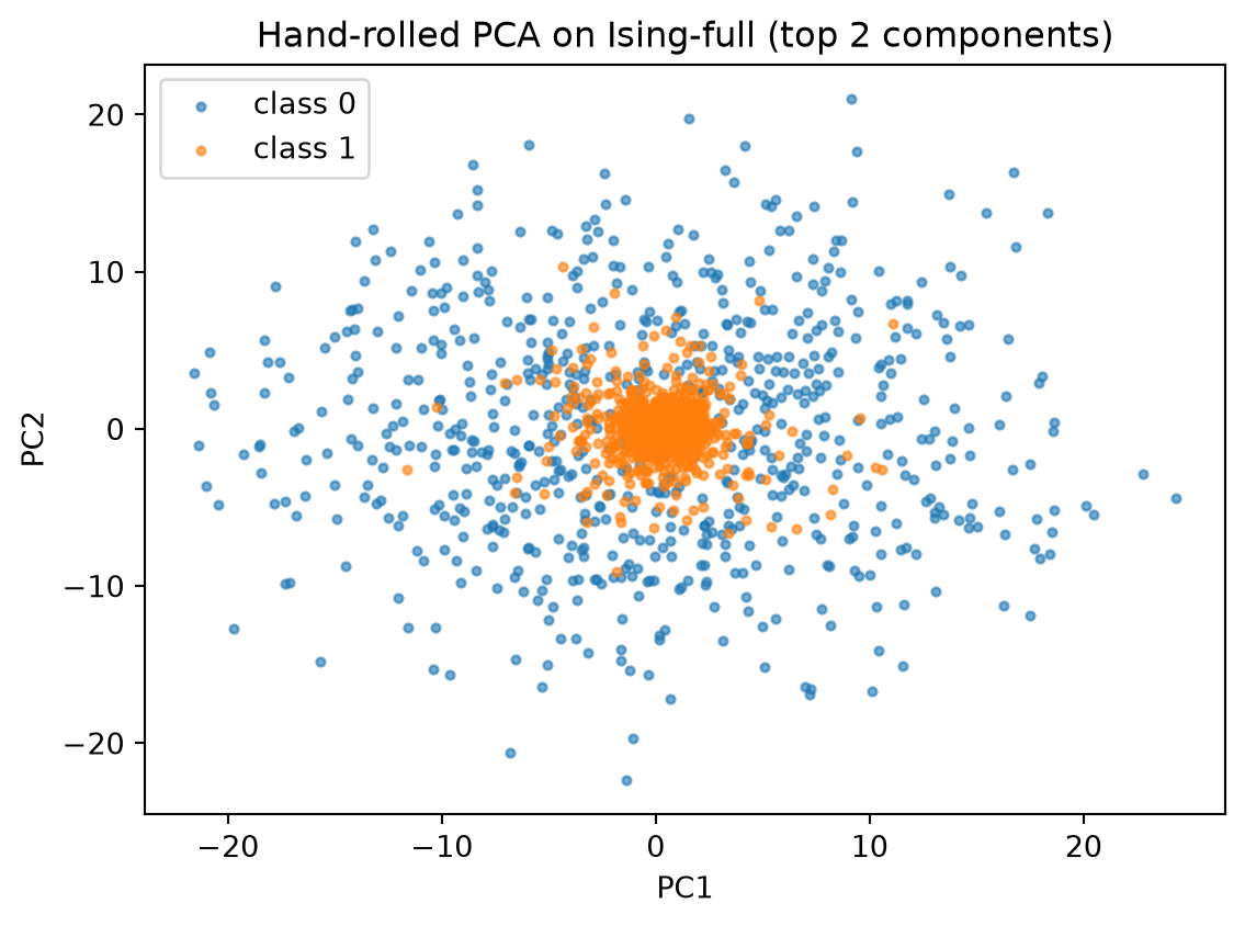
The whole of PCA is two lines once you stop fearing the covariance matrix. We compute it explicitly so you can read off where the variance lives, then project the 64×64 = 4096-D Ising images down to k principal components and reconstruct.
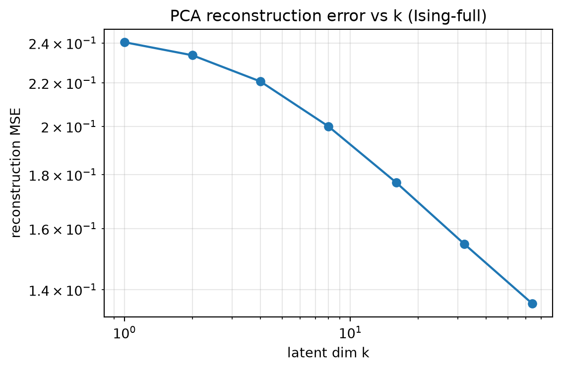
# Reconstruction error vs latent dim k. We sweep k and report MSE# averaged over the training set.ks = [1, 2, 4, 8, 16, 32, 64]mses = []for k in ks: _, X_rec, _, _ = pca_from_scratch(X_flat, k=k) mse = ((X_flat - X_rec) **2).mean().item() mses.append(mse)print(f" k = {k:3d} MSE = {mse:.5f}")fig, ax = plt.subplots(figsize=(6, 4))ax.plot(ks, mses, "o-", lw=1.6)ax.set_xscale("log"); ax.set_yscale("log")ax.set_xlabel("latent dim k"); ax.set_ylabel("reconstruction MSE")ax.set_title("PCA reconstruction error vs k (Ising-full)")ax.grid(True, which="both", alpha=0.3)plt.tight_layout(); plt.show()
  k =   1   MSE = 0.24038
  k =   2   MSE = 0.23362
  k =   4   MSE = 0.22063
  k =   8   MSE = 0.20003
  k =  16   MSE = 0.17688
  k =  32   MSE = 0.15469
  k =  64   MSE = 0.13580
Reading the curve. Reconstruction MSE decays monotonically — that’s the spectrum of the covariance matrix in disguise. The “elbow” you see (around k = 8 or so) is where additional dimensions are paying for diminishing returns. This is the linear answer to “how many degrees of freedom does the data have?”; the autoencoder we build on Thursday (Block 3) gives the nonlinear answer and usually finds a much smaller k.
Part B — t-SNE and UMAP on Ising-full latents
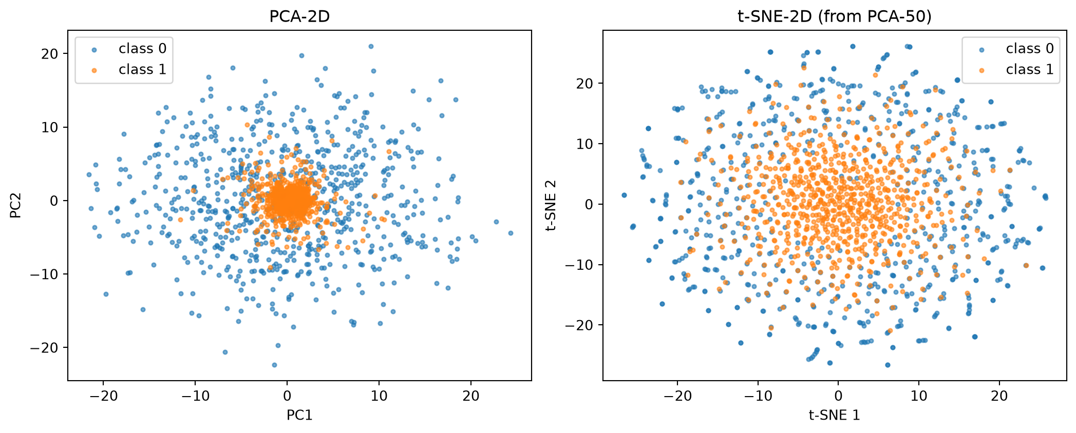
t-SNE is the most popular nonlinear visualisation of high-D data. It preserves local neighbourhood structure: two points that were near each other in the original space should end up near each other in the 2-D layout. But the converse is not true: two points that end up near each other in 2-D may have been far apart in the original space, because t-SNE exaggerates distances between separated clusters.
This is the distance trap: people read t-SNE plots as if pixel-space distance equalled t-SNE distance. It does not.
UMAP[@mcinnes_2018_umap] is the 2026 default for 2-D embeddings of materials-science feature spaces. It is built on the same fuzzy-simplicial foundation as t-SNE but trades the heavy KL-divergence optimisation for a cross-entropy on a sparse k-NN graph: faster, scalable to millions of points, and — most importantly for this exercise — it preserves more of the global structure. After running both, you should be able to see the difference.
(see MFML §“t-SNE — perplexity, t-distribution, and what it is for”, §“UMAP — the 2026 default for 2-D visualisation”, §“What latent visualisations don’t tell you”)
# Project Ising-full to 2-D with t-SNE. We project the *flattened pixels*# directly; on a real problem you would first reduce to k=50 with PCA for# speed, but on Ising-full at N=1500 the direct path is fast enough.## Using the PCA-50 path is recommended in production - it's also what the# MFML W9 lecture shows.print("Pre-reducing to PCA-50 for t-SNE...")Z50, _, _, _ = pca_from_scratch(X_flat, k=50)print("Running t-SNE on the PCA-50 features...")tsne = TSNE(n_components=2, perplexity=30, init="pca", random_state=0)Z_tsne = tsne.fit_transform(Z50.numpy())print(f"t-SNE output shape: {Z_tsne.shape}")
Pre-reducing to PCA-50 for t-SNE...
Running t-SNE on the PCA-50 features...
t-SNE output shape: (1500, 2)
# The distance trap: pick two points close in t-SNE but far in pixel space.tsne_pts = torch.tensor(Z_tsne, dtype=torch.float32)N = tsne_pts.shape[0]# Pairwise t-SNE distances and pairwise pixel distances on a 200-point sub.sub_idx = torch.randperm(N, generator=torch.Generator().manual_seed(1))[:200]d_tsne = torch.cdist(tsne_pts[sub_idx], tsne_pts[sub_idx])d_pix = torch.cdist(X_flat[sub_idx], X_flat[sub_idx])# Find a pair with t-SNE rank in the top 5% but pixel rank in the bottom 50%.flat = torch.triu_indices(d_tsne.shape[0], d_tsne.shape[1], offset=1)i_, j_ = flat[0], flat[1]d_t = d_tsne[i_, j_]; d_p = d_pix[i_, j_]t_rank = d_t.argsort().argsort().float() / d_t.numel()p_rank = d_p.argsort().argsort().float() / d_p.numel()candidates = ((t_rank <0.05) & (p_rank >0.5)) # close in t-SNE, far in pixelsif candidates.any(): pick = candidates.nonzero()[0, 0].item() a, b =int(i_[pick]), int(j_[pick])print(f"Distance-trap pair: t-SNE dist = {d_t[pick]:.2f} (rank {t_rank[pick].item():.0%}), "f"pixel dist = {d_p[pick]:.2f} (rank {p_rank[pick].item():.0%})")else:print("No clear distance-trap pair found — try perplexity or seed.")
UMAP — n_neighbors sweep, runtime, and side-by-side with t-SNE
umap-learn is not in the default course env. Install it with pip install umap-learn (wrapped in try/except like the TabPFN pattern you saw in Week 8) and re-run this cell. If the import fails the cell prints an install hint and skips — your hand-in is then just the t-SNE half plus a note that you did not get UMAP running.
What we sweep.n_neighbors is UMAP’s single most consequential hyperparameter. Small values (5) over-fragment the manifold and behave like t-SNE; large values (200) push UMAP toward a global, almost linear-looking layout. We measure runtime alongside the layout so you can feel the cost-quality knob.
import timetry:import umap # noqa: F401 (the actual API is umap.UMAP) HAVE_UMAP =TrueexceptImportError: HAVE_UMAP =Falseprint("umap-learn not installed — skipping the UMAP sweep.\n"" pip install umap-learn\n""and re-run this cell to complete Part B." )if HAVE_UMAP:import umap as umap_lib nn_values = [5, 15, 50, 200] umap_embeddings = {} umap_runtimes = {}for nn in nn_values: reducer = umap_lib.UMAP( n_components=2, n_neighbors=nn, min_dist=0.1, random_state=0, ) t0 = time.time() Z_u = reducer.fit_transform(Z50.numpy()) umap_runtimes[nn] = time.time() - t0 umap_embeddings[nn] = Z_uprint(f" UMAP n_neighbors = {nn:3d} runtime = {umap_runtimes[nn]:.2f} s")# 2x2 grid of UMAPs + the t-SNE on a 5th panel (use a 2x3 layout, leave one blank). fig, axes = plt.subplots(2, 3, figsize=(13.5, 8))for ax, nn inzip(axes.flat[:4], nn_values): Z_u = umap_embeddings[nn]for cls in [0, 1]: m = (y == cls).numpy() ax.scatter(Z_u[m, 0], Z_u[m, 1], s=8, alpha=0.6, c=f"C{cls}", label=f"class {cls}") ax.set_title(f"UMAP n_neighbors = {nn} ({umap_runtimes[nn]:.2f} s)") ax.set_xlabel("UMAP 1"); ax.set_ylabel("UMAP 2") ax.legend(fontsize=8)# Panel 5: the t-SNE we already ran, for direct comparison. ax = axes.flat[4]for cls in [0, 1]: m = (y == cls).numpy() ax.scatter(Z_tsne[m, 0], Z_tsne[m, 1], s=8, alpha=0.6, c=f"C{cls}", label=f"class {cls}") ax.set_title("t-SNE (perplexity = 30) — comparison") ax.set_xlabel("t-SNE 1"); ax.set_ylabel("t-SNE 2"); ax.legend(fontsize=8)# Panel 6: blank. axes.flat[5].axis("off") plt.suptitle("Ising-full (PCA-50 features) — UMAP n_neighbors sweep vs t-SNE", y=1.02) plt.tight_layout(); plt.show()
umap-learn not installed — skipping the UMAP sweep.
  pip install umap-learn
and re-run this cell to complete Part B.
Reflection question (write 1-2 sentences in your hand-in). Across the four UMAP panels and the t-SNE panel, which method preserves the global structure better — i.e. which one keeps the two Ising classes on a sensible relative scale rather than blowing them apart into isolated islands? Note that at low n_neighbors UMAP behaves closer to t-SNE; at high n_neighbors it pushes toward a more PCA-like global layout.
(Answer for the marker: UMAP, especially at n_neighbors ≥ 50, keeps inter-cluster distances meaningful. t-SNE’s KL objective explicitly exaggerates them. See [@mcinnes_2018_umap].)
Part C — Augmentation pipeline for contrastive learning
Contrastive learning needs positive pairs — two views of the same underlying object — and negatives — views from different objects. A “view” is just an augmented version of an image. The augmentations encode the invariances you want the latent space to respect: a model trained with rotations as positives will learn rotation-invariant features; a model trained with colour-jitter positives will learn colour-invariant features.
For Ising microstructures, the natural invariances are:
Rotation by k × 90° (the lattice has no preferred direction).
Flips (the spin-up and spin-down domains are exchangeable below T_c and the order parameter is symmetric across mirrors).
Small additive noise (we’d like the embedding to be robust to imaging noise / measurement noise).
Crucially, these augmentations preserve the class label (above vs below T_c) — that’s how we know they’re “valid invariances” for this task. No model training in this part. Just the data-prep that Thursday Block 6’s InfoNCE loop will consume.
(see MFML §“Positive-pair construction”, §“Augmentations as an implicit prior on what to make invariant”)
def make_positive_pair(x, rng=None):"""Two augmented views of the same Ising image. x: (1, H, W) float tensor in [0, 1]. Returns (xi, xj), both same shape and dtype. Augmentations applied independently to each view: - random rotation by 0/90/180/270 degrees - random horizontal flip with p=0.5 - random vertical flip with p=0.5 - additive Gaussian noise, sigma in [0.0, 0.1] """if rng isNone: rng = np.random.default_rng()def aug(t):# rotation k =int(rng.integers(0, 4)) t = torch.rot90(t, k, dims=(-2, -1))# h-flipif rng.random() <0.5: t = torch.flip(t, dims=(-1,))# v-flipif rng.random() <0.5: t = torch.flip(t, dims=(-2,))# noise sigma =float(rng.uniform(0.0, 0.1)) t = t + sigma * torch.randn_like(t)return t.clamp(0.0, 1.0)return aug(x), aug(x)
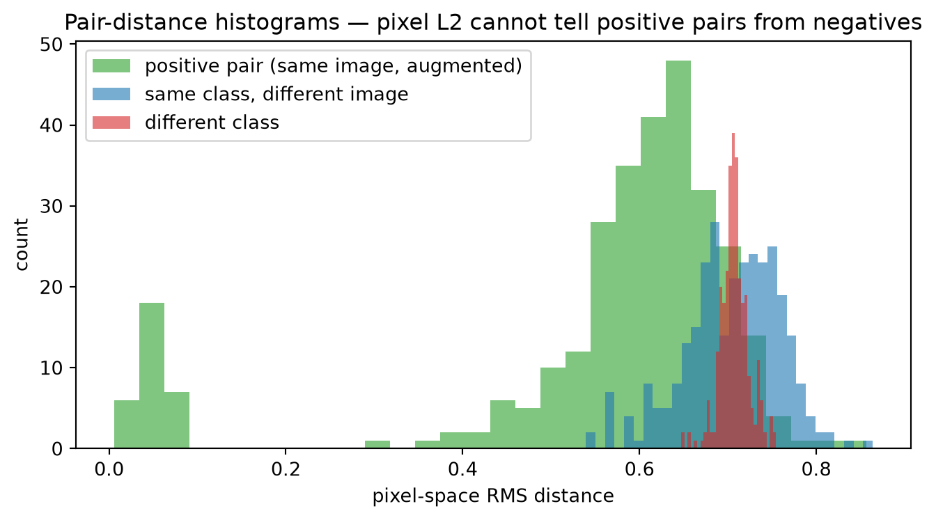
# Verify the augmentations *preserve class* but *break pixel similarity*.rng = np.random.default_rng(0)n_pairs =300intra_pos_dists = [] # pos-pair pixel L2intra_class_dists = [] # different image, same classinter_class_dists = [] # different image, different classidx0 = (y ==0).nonzero().squeeze()[:200]idx1 = (y ==1).nonzero().squeeze()[:200]# Same-image positive pairsfor i inrange(n_pairs): j =int(idx0[i %len(idx0)]) xi, xj = make_positive_pair(X_img[j], rng=rng) intra_pos_dists.append((xi - xj).pow(2).mean().sqrt().item())# Different-image, same-classfor i inrange(n_pairs): a =int(idx0[i %len(idx0)]) b =int(idx0[(i +7) %len(idx0)]) intra_class_dists.append((X_img[a] - X_img[b]).pow(2).mean().sqrt().item())# Different-image, different-classfor i inrange(n_pairs): a =int(idx0[i %len(idx0)]) b =int(idx1[i %len(idx1)]) inter_class_dists.append((X_img[a] - X_img[b]).pow(2).mean().sqrt().item())fig, ax = plt.subplots(figsize=(7, 4))ax.hist(intra_pos_dists, bins=30, alpha=0.6, label="positive pair (same image, augmented)", color="C2")ax.hist(intra_class_dists, bins=30, alpha=0.6, label="same class, different image", color="C0")ax.hist(inter_class_dists, bins=30, alpha=0.6, label="different class", color="C3")ax.set_xlabel("pixel-space RMS distance")ax.set_ylabel("count")ax.set_title("Pair-distance histograms — pixel L2 cannot tell positive pairs from negatives")ax.legend(); plt.tight_layout(); plt.show()
Reading the histogram. The three distributions overlap heavily. In pixel space, “two augmentations of the same Ising image” are not closer than “two different images of the same class”. This is precisely why we need a learned encoder — the model must discover an embedding in which positive pairs become close and unrelated images become far. That is the contrastive job description.
Part D — Reflection (1 paragraph, ~5 sentences)
Write a paragraph answering: PCA, t-SNE, and contrastive learning all produce a low-dimensional embedding of high-D data — but they answer different questions. Specifically address:
Which method is quantitative (you can compute reconstruction error in the original space)?
Which method is purely visual (the embedding axes are not interpretable, distances are not metric)?
Which method uses no labels at all for training, even implicitly?
Which method is most computationally expensive?
Reference one observation from your Part A reconstruction-error curve and one from your Part C distance histograms.
Bridge to Thursday. On Thursday the MFML tools you built here get applied to a fourth and fifth setting: synthetic XRD spectra (ML-PC — PCA + reconstruction-error anomaly scoring) and the bottleneck of a convolutional autoencoder on Ising (MFML Block 3). Your Part D paragraph should already have an opinion about which tool to pick first, and what to follow up with.
But Thursday’s MG leg asks a different question entirely — not “what does the embedding organise by?” but “is the regression number trustworthy?” That is MG Unit 8, and Part E below is its warm-up.
Part E — MG Unit 8 prep: trustworthy materials regression
Parts A–D were about geometry: what does a latent space organise by? Part E is the orthogonal MG question, and the one MG Unit 8 is built around:
In materials ML, the test set’s relationship to the training set is the scientific claim. A regression model is trustworthy only when its split design matches the claim its predictions are meant to support — and that claim is backed by a baseline ladder, per-region residuals, and an honest reporting checklist.
This is prep, not the full analysis — Thursday’s MG block (Blocks 4–5) does the heavy version. Here you build just enough machinery to walk in already fluent in the four core ideas:
leakage-safe split design (random vs CV-folds vs group-aware),
the mandatory baseline ladder (constant → linear → GBT),
a per-region residual read, and
the seven-point trustworthy-reporting checklist.
We use the real MatBenchDataset perovskites benchmark (the same one Thursday uses): ~19k DFT-relaxed perovskites, target = formation energy (eV/atom), features = a 118-D element-fraction composition vector (ds.X, ds.y). Because it is a real composition benchmark, a composition baseline does real work and the leakage question is not hypothetical. The dataset also ships 5 reproducible surrogate folds (ds.folds) — official Matbench folds need the matbench PyPI package; the surrogate folds are sufficient for split-design teaching, not for leaderboard parity. No GNN training in this homework (that is Thursday); the baselines fit in seconds on CPU on a subsample.
(see MG U8 §C “split design”, §D29 “the mandatory baseline ladder”, §E “per-region residual diagnostics”, §F47 “trustworthy-reporting checklist”)
from ai4mat.datasets import MatBenchDatasetds = MatBenchDataset(task="matbench_perovskites", download=True)# ~19k crystals make the GBT tier slow on CPU; take a seeded 4000-row# subsample. All split logic operates on this subsample._sub_rng = np.random.default_rng(0)N_MB =min(4000, len(ds.X))mb_sub = np.sort(_sub_rng.permutation(len(ds.X))[:N_MB])X_mb = np.asarray(ds.X)[mb_sub].astype(np.float64) # (N_MB, 118)y_mb = np.asarray(ds.y)[mb_sub].astype(np.float64) # (N_MB,) eV/atom# A "composition family" label derived purely from ds.X: the column of# the largest element fraction once oxygen (Z=8 -> column index 7) is# zeroed. Most of these perovskites are oxides, so this dominant# non-oxygen element is a stable, purely-compositional family key — the# chemistry-family axis MG §B10 cares about._X_no_O = X_mb.copy()_X_no_O[:, 7] =0.0family_z = _X_no_O.argmax(axis=1) +1# 1-based atomic Z# Re-index the reproducible surrogate folds onto the subsample._pos = {orig: k for k, orig inenumerate(mb_sub)}mb_folds = []for tr_o, te_o in ds.folds: tr = np.array([_pos[i] for i in tr_o if i in _pos], dtype=np.int64) te = np.array([_pos[i] for i in te_o if i in _pos], dtype=np.int64) mb_folds.append((tr, te))print(f"MatBench perovskites: using {N_MB} / {len(ds.X)} crystals; "f"{len(np.unique(family_z))} composition families; "f"{len(mb_folds)} reproducible surrogate folds.")
# The composition feature is `ds.X` directly — a 118-D element-fraction# vector, the Magpie-spirit input MG §D29 asks every baseline ladder to# stand on. No bespoke descriptor needed: real benchmark, real features.def split_random(seed=0, frac=0.8):"""IID split — probes *no* generalization axis (MG slide 20).""" rng = np.random.default_rng(seed) perm = rng.permutation(N_MB) cut =int(frac * N_MB)return perm[:cut], perm[cut:]def split_family_heldout(held_elements):"""Chemistry-aware split: every crystal whose dominant non-oxygen element is in `held_elements` (1-based atomic Z) moves to test, so chemistry-family leakage is impossible by construction (MG §B10 / §C21).TODO (1 line): return (train_idx, test_idx). `held` below is a boolean mask that is True for crystals whose family must be held out. Train = crystals NOT held; test = crystals held. """ held = np.isin(family_z, list(held_elements))# TODO: replace the next line. Hint: np.where(~held)[0], np.where(held)[0] train_idx, test_idx = np.where(~held)[0], np.where(held)[0]return train_idx, test_idx
E.1 — The mandatory baseline ladder under three split designs
The ladder is the discipline MG §D29 demands of every materials regression paper:
Tier 0 — constant (predict the training-set mean). “Anything that doesn’t beat tier 0 is broken.”
Tier 1 — composition vector + ridge (the Magpie+linear analogue).
Tier 2 — composition vector + gradient-boosted trees (the skeptic’s baseline).
Three split designs on the real benchmark: a random 80/20, the dataset’s 5 reproducible surrogate folds (ds.folds — IID-but-honest CV; official Matbench folds need the matbench pkg), and a composition-family hold-out.
A leakage rule shared by every tier: the feature standardiser is fit on train only (MG §D32 — “any operation that touches the test data before the split is leakage”). The skeleton below already does this correctly; your job is the one-line tier-0 stub.
def baseline_ladder(tr_idx, te_idx):"""{tier_name: test_MAE} on the given split. Standardiser fit on train only — do NOT change that; it is the leakage-safe contract.""" Xtr_raw, Xte_raw = X_mb[tr_idx], X_mb[te_idx] ytr, yte = y_mb[tr_idx], y_mb[te_idx] mu = Xtr_raw.mean(0, keepdims=True) # train-only fit sd = Xtr_raw.std(0, keepdims=True) +1e-8 Xtr = (Xtr_raw - mu) / sd Xte = (Xte_raw - mu) / sd out = {}# Tier 0 — constant baseline.# TODO (1 line): predict the *training* mean for every test crystal.# Hint: np.full_like(yte, ytr.mean()) const = np.full_like(yte, ytr.mean()) out["tier0_constant"] = mean_absolute_error(yte, const)# Tier 1 — ridge on the composition vector. ridge = Ridge(alpha=1.0).fit(Xtr, ytr) out["tier1_ridge"] = mean_absolute_error(yte, ridge.predict(Xte))# Tier 2 — gradient-boosted trees (the skeptic's baseline). gbt = GradientBoostingRegressor( n_estimators=200, max_depth=3, learning_rate=0.05, random_state=0, ).fit(Xtr, ytr) out["tier2_gbt"] = mean_absolute_error(yte, gbt.predict(Xte))return out# Random split (no generalization axis probed).tr_r, te_r = split_random(seed=0)ladder_random = baseline_ladder(tr_r, te_r)# ds.folds CV: average the 5 reproducible surrogate folds (the# random-vs-CV contrast — same IID regime, just de-noised).cv_fold = {k: [] for k in ladder_random}for tr_f, te_f in mb_folds:for k, mae in baseline_ladder(tr_f, te_f).items(): cv_fold[k].append(mae)ladder_cv = {k: float(np.mean(v)) for k, v in cv_fold.items()}# Composition-family hold-out: hold out the light-element family# (Z = 3 Li, 4 Be, 5 B — every crystal whose dominant non-oxygen element# is one of these moves entirely to test; ~330 crystals here).HELD_FAMILY = [3, 4, 5]tr_c, te_c = split_family_heldout(HELD_FAMILY)ladder_family = {k: mae for k, mae in baseline_ladder(tr_c, te_c).items()}print("Formation-energy MAE (eV/atom) by tier and split design")print(f"{'tier':<18}{'random':>10}{'cv (folds)':>12}{'family-held':>13}"f"{' Δ_shift (fam)':>17}")print("-"*70)for k in ladder_random: mr, mv, mc = ladder_random[k], ladder_cv[k], ladder_family[k]print(f"{k:<18}{mr:>10.4f}{mv:>12.4f}{mc:>13.4f}{mc - mr:>17.4f}")print(f"(family hold-out: {len(te_c)} test crystals; dominant non-O "f"element Z in {HELD_FAMILY})")
Formation-energy MAE (eV/atom) by tier and split design
tier                  random  cv (folds)  family-held    Δ_shift (fam)
----------------------------------------------------------------------
tier0_constant        0.5694      0.5602       0.5117          -0.0577
tier1_ridge           0.4529      0.4419       0.4893           0.0364
tier2_gbt             0.4628      0.4488       0.5157           0.0530
(family hold-out: 330 test crystals; dominant non-O element Z in [3, 4, 5])
What you should see (and put in your hand-in). The learned tiers (ridge, GBT) beat tier 0 on the random split (else they would be broken). The random number is small — it probes no generalization axis. The ds.folds CV column tracks the random number closely: CV does not probe a new axis, it only de-noises the IID estimate (and these are surrogate folds — fine for split-design teaching, not leaderboard parity). The composition-family split inflates the learned-tier MAE: the gap between the family number and the random/CV number is the fourth bias-variance term \(\Delta_\text{shift}\) (MG slide 05) — pure distribution-shift error; bias, variance, and noise did not change, the training distribution did. On a real benchmark this gap is honest and often modest (a 118-D composition vector transfers reasonably across chemistries) — and tier 0 can even improve on the held family if that family’s energies are low-variance, which is exactly why tier 0 is a floor, not a model. Reporting the gap, modest or not, is the discipline.
Hand-in question (one line).You want to claim your model discovers stable perovskites in chemistry it has never seen. Which split gives the honest headline number for that claim, and which one would be the “random-split numbers in a discovery-claim paper” anti-pattern?
(Answer for the marker: the composition-family-held-out split is the honest headline for a new-chemistry discovery claim; reporting only the random or surrogate-CV number for that claim is the MG slide-48 anti-pattern. The random/CV pair answers an in-distribution claim instead.)
E.2 — A per-region residual read
A single global MAE hides where a materials model fails (MG §E — “global MAE hides localized failure”). The minimum honest diagnostic is a per-family residual table: for each composition family, the test MAE and the signed bias (mean of true − pred; a non-zero value means the model systematically over- or under-shoots that family).
We use the tier-1 ridge on the random split as the worked regressor (cheap, and on this real benchmark it is competitive with the GBT tier).
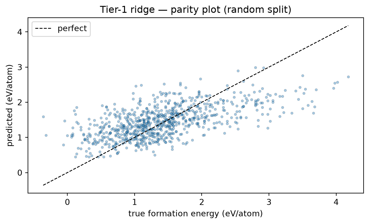
mu = X_mb[tr_r].mean(0, keepdims=True)sd = X_mb[tr_r].std(0, keepdims=True) +1e-8ridge_e = Ridge(alpha=1.0).fit((X_mb[tr_r] - mu) / sd, y_mb[tr_r])pred_te = ridge_e.predict((X_mb[te_r] - mu) / sd)true_te = y_mb[te_r]# Report the five most common composition families in the test set.fam_te = family_z[te_r]top_fam = [z for z, _ insorted(zip(*np.unique(fam_te, return_counts=True)), key=lambda zc: -zc[1])][:5]print("Per-family residuals — tier-1 ridge, random split (MG §E38)")print(f"{'family Z':<10}{'N_test':>7}{'MAE':>10}{'signed bias':>14}")print("-"*41)for z in top_fam: m = fam_te == z mae_p = mean_absolute_error(true_te[m], pred_te[m])# TODO (1 line): signed bias = mean of (true - pred) on this family.# Hint: float((true_te[m] - pred_te[m]).mean()) bias_p =float((true_te[m] - pred_te[m]).mean())print(f"Z={int(z):<8}{int(m.sum()):>7}{mae_p:>10.4f}{bias_p:>+14.4f}")print(f"{'GLOBAL':<10}{len(te_r):>7}"f"{mean_absolute_error(true_te, pred_te):>10.4f}"f"{float((true_te - pred_te).mean()):>+14.4f}")fig, ax = plt.subplots(figsize=(6.5, 4))ax.scatter(true_te, pred_te, s=10, alpha=0.4, edgecolor="k", lw=0.2)lims = [true_te.min(), true_te.max()]ax.plot(lims, lims, "k--", lw=1, label="perfect")ax.set_xlabel("true formation energy (eV/atom)")ax.set_ylabel("predicted (eV/atom)")ax.set_title("Tier-1 ridge — parity plot (random split)")ax.legend(); plt.tight_layout(); plt.show()
Per-family residuals — tier-1 ridge, random split (MG §E38)
family Z   N_test       MAE   signed bias
-----------------------------------------
Z=7           432    0.4630       -0.0313
Z=9           109    0.4670       -0.0166
Z=16           72    0.4022       -0.0452
Z=3            26    0.3742       -0.1679
Z=5            21    0.4804       -0.0450
GLOBAL        800    0.4529       -0.0346
Reading the residual table. The global MAE is one number; the per-family rows tell you whether the model is uniformly OK or whether it is carried by a few easy chemistries and quietly wrong on the rest. A large per-family signed bias is the localized-failure signature MG §E is built around — and it is invisible in the global MAE. (You will extend this on Thursday with the OOD distance-to-train diagnostic and a bootstrap CI.)
E.3 — Score this against the 7-point checklist
MG Unit 8 closes (§F47) with a seven-point trustworthy-reporting checklist. The afternoon MG exercise is graded against it (target: 5/7). Score this Part E by filling the Status column in your hand-in:
#
Checklist item
Did Part E do it?
1
Split design declared & matched to the claim
? — we ran random, ds.folds CV and a composition-family hold-out and discussed which matches a discovery claim
2
Mandatory baselines (constant, linear, GBT)
? — tiers 0/1/2 ladder on the real benchmark
3
Per-region residuals (per-family table)
? — per-composition-family MAE + signed bias
4
Structure-awareness ablation
? — N/A on a composition-only benchmark (Thursday Block 5b does the edge-scramble ablation on the synthetic graph)
? — family-disjoint splits; standardiser fit on train only
6
Confidence interval on the headline MAE
? — not in this homework (Thursday Block 5 adds the bootstrap CI)
7
Test-set construction documented
? — real Matbench matbench_perovskites; seeded subsample of a fixed snapshot; family-disjoint split. Official folds need the matbench pkg; we use the dataset’s reproducible surrogate folds and say so
Hand-in (one line). Replace each “?” with ✅ / ◻️ and report your Part E score out of 7. Then state, in one sentence, which missing items Thursday’s MG block must add to reach the exercise’s 5/7 bar.
(Answer for the marker: Part E scores 5/7 — items 1, 2, 3, 5, 7 are met; item 6 (bootstrap CI) is added by Thursday’s Block 5 and item 4 (structure-awareness ablation) by the Block-5b synthetic appendix (it is N/A on a composition-only benchmark — nothing to scramble). The MG sentence to leave with: better features or a fancier architecture never fix bad benchmarking — the split is part of the hypothesis, not the postprocessing.)
You’re done with Week 9 homework. Bring your five deliverables on Thursday:
PCA reconstruction error vs latent dim curve (Part A).
t-SNE 2-D plot with the distance-trap pair annotated (Part B).
Pixel-distance histogram for positive vs negative pairs (Part C).
Method-comparison paragraph (Part D).
The random / CV / family MAE table + Δ_shift, your split-choice answer, the per-family residual table, and your 7-point checklist score (Part E).