import json
import time
import warnings
from pathlib import Path

import matplotlib.pyplot as plt
import numpy as np
import pandas as pd

warnings.filterwarnings('ignore')

from sklearn.ensemble import RandomForestRegressor
from sklearn.kernel_ridge import KernelRidge
from sklearn.decomposition import PCA
from sklearn.inspection import permutation_importance
from sklearn.metrics import mean_absolute_error
from sklearn.model_selection import GroupShuffleSplit, train_test_split
from sklearn.preprocessing import StandardScaler

from pymatgen.core import Composition, Structure

from matminer.featurizers.composition import ElementProperty
from matminer.featurizers.site import CrystalNNFingerprint
from matminer.featurizers.structure import (
    BondFractions,
    SiteStatsFingerprint,
)

from dscribe.descriptors import SOAP

RNG = 0
np.random.seed(RNG)SS26 Materials Genomics, FAU Erlangen (Prof. Pelz). Exercise notebook for Unit 6. Climb the descriptor ladder on a ~220-row Materials Project spinel subset:
| Tier | Descriptor | Library | Cells |
|---|---|---|---|
| 1 | Magpie composition statistics | matminer | Part 1 |
| 2 | matminer structure features (CrystalNN, BondFractions) | matminer | Part 2 |
| 3 | SOAP (atom-centred, smooth) | dscribe | Part 3 |
| – | Permutation-importance + leakage audit | scikit-learn | Part 4 |
Target. PBE band gap (eV) from matbench_mp_gap. The CSV is shipped in this folder (spinels_mp.csv, 220 entries, AB\(_2\)O\(_4\) stoichiometry, 115 distinct formulas, 105 of them with two polymorphs).
Time budget. 90 minutes total — 5 setup / 25 Part 1 / 25 Part 2 / 25 Part 3 / 15 Part 4. Parts 1–4 each re-load from the CSV in their opening cell, so you can skip ahead if you fall behind.
Part 0 — Setup (≈5 min)
Imports, version check, dataset load, sanity sniff.
In [1]:
In [2]:
from importlib.metadata import version as _v

for pkg in ['numpy', 'pandas', 'matplotlib', 'scikit-learn',
            'pymatgen', 'matminer', 'dscribe']:
    try:
        print(f'{pkg:15s} {_v(pkg)}')
    except Exception as e:
        print(f'{pkg:15s} NOT INSTALLED ({e})')
numpy 1.26.4
pandas 2.3.0
matplotlib 3.10.3
scikit-learn 1.7.0
pymatgen 2026.5.4
matminer 0.10.1
dscribe 2.1.2In [3]:
CSV = Path('spinels_mp.csv')
assert CSV.exists(), f'expected {CSV.resolve()} — see README_week06.md'

df = pd.read_csv(CSV)
df['structure'] = df['structure'].apply(lambda s: Structure.from_dict(json.loads(s)))
df['composition'] = df['pretty_formula'].apply(Composition)

print(f'dataset size:           {len(df)}')
print(f'unique formulas:        {df.pretty_formula.nunique()}')
print(f'polymorph-formulas:     {int((df.pretty_formula.value_counts() >= 2).sum())}')
print(f'band-gap range (eV):    [{df.band_gap.min():.2f}, {df.band_gap.max():.2f}]')
print(f'mean band gap:          {df.band_gap.mean():.3f} eV')
df.head(3)[['material_id', 'pretty_formula', 'band_gap', 'spacegroup']]
dataset size: 220
unique formulas: 115
polymorph-formulas: 105
band-gap range (eV): [0.00, 5.11]
mean band gap: 1.241 eV| material_id | pretty_formula | band_gap | spacegroup | |
|---|---|---|---|---|
| 0 | mb_mpgap_0000 | MgMn2O4 | 0.5791 | 13 |
| 1 | mb_mpgap_0001 | MgMn2O4 | 0.7655 | 14 |
| 2 | mb_mpgap_0002 | CaMn2O4 | 1.2826 | 141 |
In [4]:
# Sniff one structure to confirm round-trip.
ex = df.iloc[0]
print(f"{ex.pretty_formula}  (spacegroup {ex.spacegroup}, gap {ex.band_gap:.2f} eV)")
print(ex.structure)
MgMn2O4 (spacegroup 13, gap 0.58 eV)
Full Formula (Mg4 Mn8 O16)
Reduced Formula: MgMn2O4
abc : 6.026773 5.150628 11.768915
angles: 90.000000 119.066959 90.000000
pbc : True True True
Sites (28)
# SP a b c
--- ---- -------- -------- --------
0 Mg 0 0.148683 0.75
1 Mg 0 0.851317 0.25
2 Mg 0.5 0.511308 0.25
3 Mg 0.5 0.488692 0.75
4 Mn 0.765334 0.488393 0.015557
5 Mn 0.234666 0.488393 0.484443
6 Mn 0.234666 0.511607 0.984443
7 Mn 0.765334 0.511607 0.515557
8 Mn 0.5 0 0
9 Mn 0.5 0 0.5
10 Mn 0 0 0
11 Mn 0 0 0.5
12 O 0.843053 0.141912 0.101583
13 O 0.156947 0.141912 0.398417
14 O 0.156947 0.858088 0.898417
15 O 0.843053 0.858088 0.601583
16 O 0.649467 0.76553 0.896718
17 O 0.350533 0.76553 0.603282
18 O 0.350533 0.23447 0.103282
19 O 0.649467 0.23447 0.396718
20 O 0.365345 0.318117 0.881331
21 O 0.634655 0.318117 0.618669
22 O 0.127668 0.69082 0.112173
23 O 0.872332 0.69082 0.387827
24 O 0.634655 0.681883 0.118669
25 O 0.365345 0.681883 0.381331
26 O 0.872332 0.30918 0.887827
27 O 0.127668 0.30918 0.612173In [5]:
fig, ax = plt.subplots(1, 2, figsize=(10, 3.2))
ax[0].hist(df['band_gap'], bins=30, color='C0', edgecolor='k')
ax[0].set_xlabel('PBE band gap (eV)'); ax[0].set_ylabel('count')
ax[0].set_title('Target distribution')

poly_counts = df.pretty_formula.value_counts().value_counts().sort_index()
ax[1].bar(poly_counts.index.astype(int), poly_counts.values, color='C2', edgecolor='k')
ax[1].set_xlabel('# polymorphs of a given formula in dataset')
ax[1].set_ylabel('# distinct formulas')
ax[1].set_title('Polymorph multiplicity')
plt.tight_layout(); plt.show()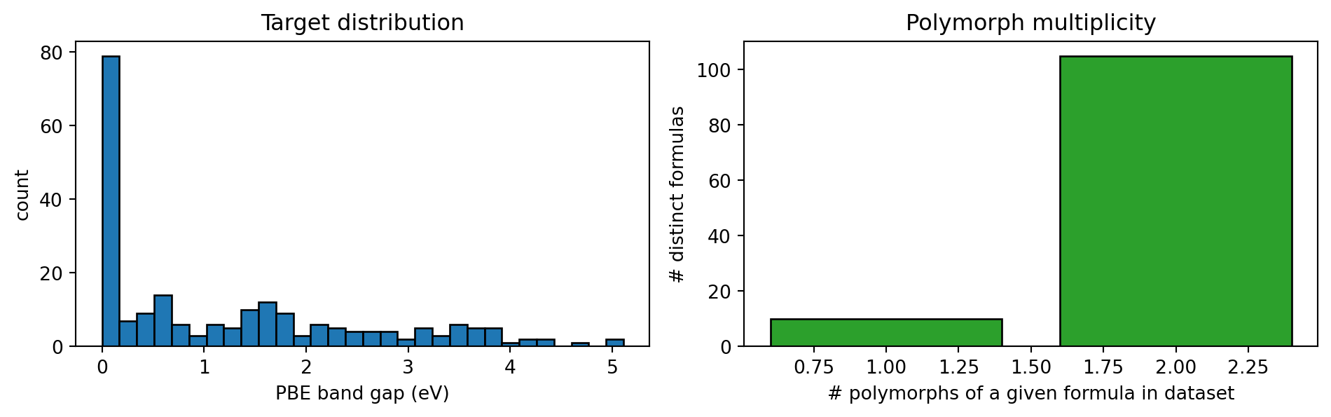
Why the polymorph-multiplicity histogram matters. 105 of the 115 distinct formulas appear with two structural polymorphs. That makes this dataset a miniature stress test for the polymorph-leakage audit in Part 4: a naive row-wise train/test split will put one polymorph of MgMn\(_2\)O\(_4\) in train and the other in test — and the model will look better than it really is. We will keep the splits grouped by formula throughout Parts 1–3 and break that rule deliberately in Part 4.
In [6]:
# Container for results across all parts — populated as we go.
results: dict[str, dict] = {}

def report(name: str, mae: float, t_train: float, n_features: int) -> None:
    results[name] = dict(mae=mae, t_train=t_train, n_features=n_features)
    print(f'{name:22s}  MAE = {mae:.3f} eV   '
          f'train = {t_train:6.2f}s   features = {n_features}')
Part 1 — Magpie composition baseline (≈25 min, must-finish)
Magpie elemental statistics (Ward 2016) are the tier-1 descriptor: they ignore structure entirely and just summarise the elements present. For bulk-thermodynamic targets this is embarrassingly competitive — and it is the floor every structure-aware claim should clear before celebrating.
We split by formula group so that polymorphs of the same compound can never land in both train and test. GroupShuffleSplit on pretty_formula does exactly that.
In [7]:
# This cell is self-contained: it reloads the CSV so Part 1 runs even
# if you skipped Part 0. (Each Part has the same idiom.)
if 'df' not in globals():
    df_local = pd.read_csv('spinels_mp.csv')
    df_local['structure'] = df_local['structure'].apply(
        lambda s: Structure.from_dict(json.loads(s)))
    df_local['composition'] = df_local['pretty_formula'].apply(Composition)
else:
    df_local = df

ep = ElementProperty.from_preset('magpie')
print(f'Magpie produces {len(ep.feature_labels())} features per composition.')

t0 = time.perf_counter()
X_magpie = ep.featurize_many(df_local['composition'].tolist(),
                              ignore_errors=True, pbar=False)
X_magpie = np.array(X_magpie, dtype=float)
print(f'featurise time: {time.perf_counter() - t0:.1f}s')
print(f'feature matrix: {X_magpie.shape}')
Magpie produces 132 features per composition.
featurise time: 0.5s
feature matrix: (220, 132)In [8]:
# Drop any all-NaN columns (rare; matminer can return NaN for elements
# with missing tabulated properties — none for d-block oxides, but be safe).
finite_mask = np.isfinite(X_magpie).all(axis=0)
X_magpie = X_magpie[:, finite_mask]
magpie_names = [n for n, k in zip(ep.feature_labels(), finite_mask) if k]
y = df_local['band_gap'].to_numpy()
groups = df_local['pretty_formula'].to_numpy()
print(f'after NaN-column drop: {X_magpie.shape}')
after NaN-column drop: (220, 132)In [9]:
gss = GroupShuffleSplit(n_splits=1, test_size=0.25, random_state=RNG)
train_idx, test_idx = next(gss.split(X_magpie, y, groups=groups))

# Verify no formula leaks across the split.
train_formulas = set(groups[train_idx])
test_formulas = set(groups[test_idx])
leak = train_formulas & test_formulas
print(f'train: {len(train_idx)}  test: {len(test_idx)}')
print(f'leak (formulas in both): {len(leak)}  (must be 0)')
assert len(leak) == 0
train: 165 test: 55
leak (formulas in both): 0 (must be 0)In [10]:
t0 = time.perf_counter()
rf1 = RandomForestRegressor(n_estimators=200, random_state=RNG, n_jobs=-1)
rf1.fit(X_magpie[train_idx], y[train_idx])
t_train_1 = time.perf_counter() - t0

y_pred_1 = rf1.predict(X_magpie[test_idx])
MAE_1 = mean_absolute_error(y[test_idx], y_pred_1)
report('1 Magpie comp', MAE_1, t_train_1, X_magpie.shape[1])
1 Magpie comp MAE = 0.669 eV train = 0.33s features = 132Checkpoint. If your MAE_1 is much below 0.6 eV, your split is probably leaking — verify the assert two cells above. Typical numbers on this dataset under a grouped split are 0.7–0.9 eV; a random split collapses this to 0.4–0.5 eV by spotting the formula directly. We will prove that drop is illusory in Part 4.
In [11]:
fig, ax = plt.subplots(figsize=(4.4, 4.4))
ax.scatter(y[test_idx], y_pred_1, alpha=0.7, edgecolor='k', s=22)
lo, hi = y.min(), y.max()
ax.plot([lo, hi], [lo, hi], 'k--', lw=1)
ax.set_xlabel('true gap (eV)'); ax.set_ylabel('predicted gap (eV)')
ax.set_title(f'Tier 1 — Magpie / RF   MAE = {MAE_1:.3f} eV')
ax.set_aspect('equal'); plt.tight_layout(); plt.show()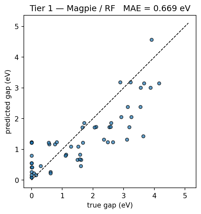
Part 2 — Add matminer structure features (≈25 min, stretch)
Tier 2 climbs one rung: we keep Magpie, but also aggregate per-site geometry into structure-level features.
SiteStatsFingerprintoverCrystalNNFingerprint("ops")— coordination / order-parameter statistics per site, then mean+std-pooled over the structure. ~122 features.BondFractions— fractional populations of element-pair bonds.
The point: same Magpie vector for all polymorphs of MgMn\(_2\)O\(_4\), but different structure-feature vectors. If structure is doing real work on this dataset, the MAE should drop.
In [12]:
if 'df' not in globals():
    df_local = pd.read_csv('spinels_mp.csv')
    df_local['structure'] = df_local['structure'].apply(
        lambda s: Structure.from_dict(json.loads(s)))
    df_local['composition'] = df_local['pretty_formula'].apply(Composition)
else:
    df_local = df

structs = df_local['structure'].tolist()
y = df_local['band_gap'].to_numpy()
groups = df_local['pretty_formula'].to_numpy()
In [13]:
# CrystalNNFingerprint("ops") site-fingerprint → mean/std pooled per structure.
ssf = SiteStatsFingerprint(
    CrystalNNFingerprint.from_preset('ops'),
    stats=('mean', 'std_dev'),
)
ssf.set_n_jobs(1)  # CrystalNN can hit thread-safety bugs in parallel

t0 = time.perf_counter()
X_ssf = ssf.featurize_many(structs, ignore_errors=True, pbar=False)
X_ssf = np.array(X_ssf, dtype=float)
print(f'SiteStatsFingerprint: {time.perf_counter() - t0:.1f}s, shape {X_ssf.shape}')
SiteStatsFingerprint: 63.4s, shape (220, 122)In [14]:
# BondFractions — but only after the featurizer has *seen* the dataset
# (it must enumerate the bond vocabulary first).
bf = BondFractions()
bf.fit(structs)
bf.set_n_jobs(1)

t0 = time.perf_counter()
X_bf = bf.featurize_many(structs, ignore_errors=True, pbar=False)
X_bf = np.array(X_bf, dtype=float)
print(f'BondFractions: {time.perf_counter() - t0:.1f}s, shape {X_bf.shape}')
BondFractions: 29.4s, shape (220, 214)In [15]:
# Stack: Magpie + CrystalNN-OPs + BondFractions.
X_struct = np.hstack([X_magpie, X_ssf, X_bf])
struct_names = (
    magpie_names
    + [f'ssf::{n}' for n in ssf.feature_labels()]
    + [f'bf::{n}' for n in bf.feature_labels()]
)
finite = np.isfinite(X_struct).all(axis=0)
X_struct = X_struct[:, finite]
struct_names = [n for n, k in zip(struct_names, finite) if k]
print(f'combined feature matrix: {X_struct.shape}')
combined feature matrix: (220, 468)In [16]:
gss = GroupShuffleSplit(n_splits=1, test_size=0.25, random_state=RNG)
train_idx, test_idx = next(gss.split(X_struct, y, groups=groups))

t0 = time.perf_counter()
rf2 = RandomForestRegressor(n_estimators=200, random_state=RNG, n_jobs=-1)
rf2.fit(X_struct[train_idx], y[train_idx])
t_train_2 = time.perf_counter() - t0

y_pred_2 = rf2.predict(X_struct[test_idx])
MAE_2 = mean_absolute_error(y[test_idx], y_pred_2)
report('2 Magpie+struct', MAE_2, t_train_2, X_struct.shape[1])
2 Magpie+struct MAE = 0.748 eV train = 0.69s features = 468Worked example — same formula, different structure. The dataset is built so that most formulas appear twice. The cell below picks one such formula, prints the two polymorphs’ (spacegroup, band gap), and prints Tier-1 and Tier-2 predictions for each. Tier 1 collapses to a single value (the Magpie vector is identical for both rows); Tier 2 can separate them — if structure features are doing useful work.
In [17]:
vc = df_local['pretty_formula'].value_counts()
poly_formulas = vc[vc >= 2].index.tolist()

# Pick the first formula whose two polymorphs straddle a band-gap gap.
chosen = None
for f in poly_formulas:
    rows = df_local[df_local['pretty_formula'] == f]
    if rows['band_gap'].max() - rows['band_gap'].min() > 0.5:
        chosen = f
        break
chosen = chosen or poly_formulas[0]
print(f'Polymorph pair: {chosen}\n')

rows = df_local[df_local['pretty_formula'] == chosen]
rows_idx = rows.index.to_numpy()
p1 = rf1.predict(X_magpie[rows_idx])
p2 = rf2.predict(X_struct[rows_idx])

out = rows[['material_id', 'spacegroup', 'band_gap']].copy()
out['pred_tier1_magpie']   = np.round(p1, 3)
out['pred_tier2_struct']   = np.round(p2, 3)
out
Polymorph pair: MnV2O4
| material_id | spacegroup | band_gap | pred_tier1_magpie | pred_tier2_struct | |
|---|---|---|---|---|---|
| 158 | mb_mpgap_0158 | 227 | 1.4876 | 1.159 | 1.217 |
| 159 | mb_mpgap_0159 | 62 | 0.8494 | 1.159 | 0.906 |
Part 3 — SOAP via dscribe (≈25 min, reach goal)
Tier 3 looks at the local atomic environment of each site. SOAP (Bartók et al. 2013) expands the smooth neighbour density around an atom into radial basis × spherical harmonics and forms a rotation- invariant power spectrum. We pass average="inner" so dscribe returns one vector per structure (averaging the rotation-invariant power spectrum across sites is itself rotation-invariant).
In [18]:
if 'df' not in globals():
    df_local = pd.read_csv('spinels_mp.csv')
    df_local['structure'] = df_local['structure'].apply(
        lambda s: Structure.from_dict(json.loads(s)))
else:
    df_local = df

structs = df_local['structure'].tolist()
y = df_local['band_gap'].to_numpy()
groups = df_local['pretty_formula'].to_numpy()

# Universe of species across the dataset (SOAP needs a fixed alphabet).
species = sorted({el.symbol for s in structs for el in s.composition.elements})
print(f'{len(species)} species in dataset: {species}')
50 species in dataset: ['Ag', 'Al', 'Au', 'Ba', 'Be', 'Bi', 'Ca', 'Cd', 'Ce', 'Co', 'Cr', 'Cu', 'Dy', 'Eu', 'Fe', 'Ga', 'Gd', 'H', 'In', 'K', 'La', 'Li', 'Lu', 'Mg', 'Mn', 'Mo', 'Na', 'Nb', 'Nd', 'Ni', 'O', 'Pr', 'Rb', 'Rh', 'Sb', 'Sc', 'Se', 'Si', 'Sm', 'Sn', 'Sr', 'Te', 'Ti', 'Tl', 'Tm', 'U', 'V', 'Y', 'Zn', 'Zr']In [19]:
# pymatgen Structure → ase.Atoms for dscribe.
from pymatgen.io.ase import AseAtomsAdaptor

ase_adaptor = AseAtomsAdaptor()
atoms_list = [ase_adaptor.get_atoms(s) for s in structs]
print(f'converted {len(atoms_list)} structures to ase.Atoms')
converted 220 structures to ase.AtomsIn [20]:
soap = SOAP(
    species=species,
    r_cut=5.0,
    n_max=6,
    l_max=4,
    periodic=True,
    average='inner',
    sparse=False,
)
print(f'SOAP descriptor dimension per structure: {soap.get_number_of_features()}')

t0 = time.perf_counter()
X_soap = soap.create(atoms_list, n_jobs=1)
t_soap = time.perf_counter() - t0
print(f'SOAP compute: {t_soap:.1f}s, shape {X_soap.shape}')
SOAP descriptor dimension per structure: 225750
SOAP compute: 0.7s, shape (220, 225750)In [21]:
# PCA-reduce: SOAP is high-dimensional and most directions carry no signal
# on a 220-row dataset. 64 components is a sensible default.
scaler = StandardScaler()
X_soap_s = scaler.fit_transform(X_soap)
n_pca = min(64, X_soap_s.shape[0] - 1, X_soap_s.shape[1])
pca = PCA(n_components=n_pca, random_state=RNG)
X_soap_pca = pca.fit_transform(X_soap_s)
print(f'PCA-reduced SOAP shape: {X_soap_pca.shape}')
print(f'explained variance (cumulative): {pca.explained_variance_ratio_.sum():.3f}')
PCA-reduced SOAP shape: (220, 64)
explained variance (cumulative): 0.550In [22]:
gss = GroupShuffleSplit(n_splits=1, test_size=0.25, random_state=RNG)
train_idx, test_idx = next(gss.split(X_soap_pca, y, groups=groups))

# (a) Kernel ridge with an RBF on SOAP-PCA.
t0 = time.perf_counter()
krr = KernelRidge(kernel='rbf', alpha=1e-2, gamma=1.0 / X_soap_pca.shape[1])
krr.fit(X_soap_pca[train_idx], y[train_idx])
t_train_3a = time.perf_counter() - t0
y_pred_3a = krr.predict(X_soap_pca[test_idx])
MAE_3a = mean_absolute_error(y[test_idx], y_pred_3a)
report('3a SOAP / KRR', MAE_3a, t_train_3a, X_soap_pca.shape[1])

# (b) Random forest on the same SOAP-PCA features, for apples-to-apples.
t0 = time.perf_counter()
rf3 = RandomForestRegressor(n_estimators=200, random_state=RNG, n_jobs=-1)
rf3.fit(X_soap_pca[train_idx], y[train_idx])
t_train_3b = time.perf_counter() - t0
y_pred_3b = rf3.predict(X_soap_pca[test_idx])
MAE_3b = mean_absolute_error(y[test_idx], y_pred_3b)
report('3b SOAP / RF', MAE_3b, t_train_3b, X_soap_pca.shape[1])
3a SOAP / KRR MAE = 1.634 eV train = 0.06s features = 64
3b SOAP / RF MAE = 1.119 eV train = 0.49s features = 64Observation, to discuss in your write-up.
SOAP captures the local atomic environment: who sits next to whom at what radial+angular distribution. matminer’s SiteStatsFingerprint captures aggregate per-site statistics — coarser but cheaper. Which won on this dataset? If SOAP did not beat Tier 2, that is a teaching moment too: the spinel subset is composition-dominated (only 115 distinct formulas, narrow chemistry), and structure-information adds little once you have decent composition+coordination features.
That is the whole point of climbing the descriptor ladder one rung at a time and reporting every rung.
Part 4 — Audit (≈15 min, critical)
This is the part that separates careful work from confident-looking nonsense. Three checks:
- Permutation importance on the best Tier-1/2/3 model — does the dominant feature make physical sense?
- Polymorph leakage — what happens if you replace
GroupShuffleSplitwith a row-wisetrain_test_split? - Tier table — collect MAEs and training times into a single table, save to
results.csv.
4.1 Permutation importance on the best model
We probe whichever model gave the lowest test MAE.
In [23]:
best_name = min(['1 Magpie comp', '2 Magpie+struct', '3a SOAP / KRR', '3b SOAP / RF'],
                key=lambda k: results[k]['mae'])
print(f'best model: {best_name}')

if best_name == '1 Magpie comp':
    X_best, model_best, names_best = X_magpie, rf1, magpie_names
elif best_name == '2 Magpie+struct':
    X_best, model_best, names_best = X_struct, rf2, struct_names
elif best_name == '3a SOAP / KRR':
    X_best, model_best, names_best = X_soap_pca, krr, [f'soap_pc{i}' for i in range(X_soap_pca.shape[1])]
else:
    X_best, model_best, names_best = X_soap_pca, rf3, [f'soap_pc{i}' for i in range(X_soap_pca.shape[1])]

gss = GroupShuffleSplit(n_splits=1, test_size=0.25, random_state=RNG)
train_idx, test_idx = next(gss.split(X_best, y, groups=groups))

t0 = time.perf_counter()
pi = permutation_importance(model_best, X_best[test_idx], y[test_idx],
                             n_repeats=8, random_state=RNG, n_jobs=-1)
print(f'permutation-importance time: {time.perf_counter() - t0:.1f}s')

order = np.argsort(pi.importances_mean)[::-1][:10]
fig, ax = plt.subplots(figsize=(7, 3.5))
ax.barh(range(len(order)),
        pi.importances_mean[order][::-1],
        xerr=pi.importances_std[order][::-1],
        color='C3', edgecolor='k')
ax.set_yticks(range(len(order)))
ax.set_yticklabels([names_best[i] for i in order[::-1]], fontsize=8)
ax.set_xlabel('mean drop in score after permutation')
ax.set_title(f'Top-10 features — {best_name}')
plt.tight_layout(); plt.show()
best model: 1 Magpie comp
permutation-importance time: 16.5s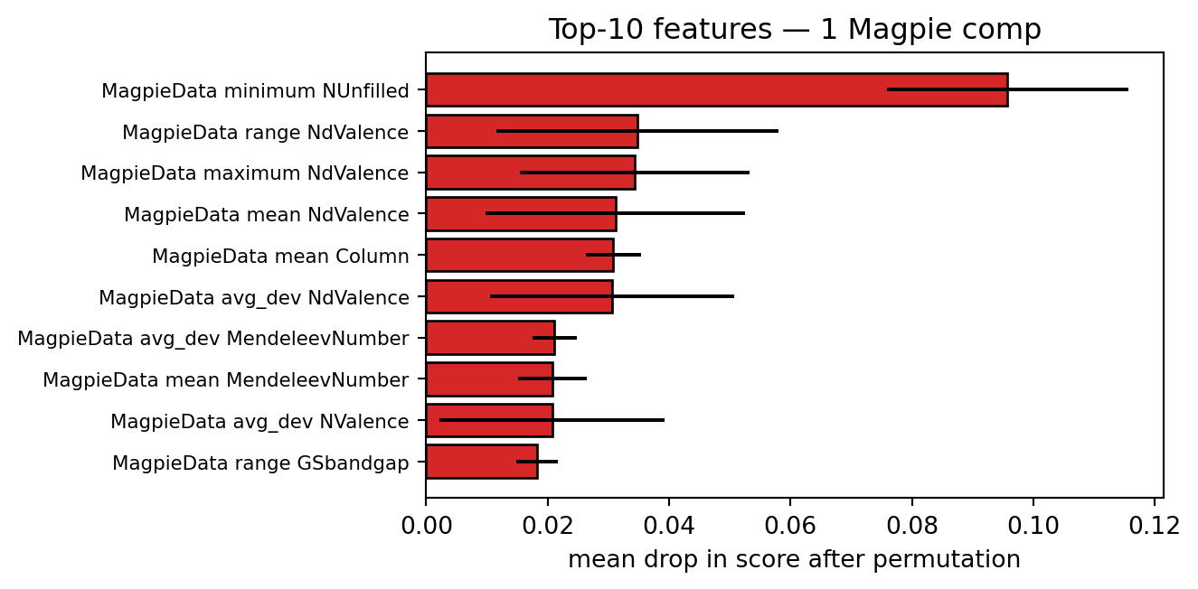
4.2 TODO — interpret the importance plot
TODO. Look at the top 5 features above and write 2–4 sentences in this markdown cell answering:
- Does the dominant feature make physical sense? e.g. for band-gap prediction we expect mean / max electronegativity, mean valence, ionic radius or band-related elemental properties to dominate. A Voronoi- or BondFraction-derived feature dominating would be more surprising — and worth a sentence on why.
- Is there a feature you do not recognise? matminer feature names are verbose but self-documenting; look up anything unfamiliar at https://hackingmaterials.lbl.gov/matminer/featurizer_summary.html.
(Replace this paragraph with your answer.)
4.3 Polymorph-leakage stress test
Re-run Part 1 with a random row-wise split (no GroupShuffleSplit). Same model, same features, different split rule — see how much MAE “improves” purely from the model being shown one polymorph at training time and asked to predict the other at test time.
In [24]:
tr_idx_r, te_idx_r = train_test_split(np.arange(len(y)), test_size=0.25, random_state=RNG)
rf1r = RandomForestRegressor(n_estimators=200, random_state=RNG, n_jobs=-1)
rf1r.fit(X_magpie[tr_idx_r], y[tr_idx_r])
MAE_1_random = mean_absolute_error(y[te_idx_r], rf1r.predict(X_magpie[te_idx_r]))

leak_count = len(set(groups[tr_idx_r]) & set(groups[te_idx_r]))
print(f'random split: train {len(tr_idx_r)}, test {len(te_idx_r)}')
print(f'leak (formulas in both halves): {leak_count}')
print(f'MAE (grouped split, Part 1): {MAE_1:.3f} eV')
print(f'MAE (random split):          {MAE_1_random:.3f} eV')
print(f'gap:                          {MAE_1 - MAE_1_random:.3f} eV')
random split: train 165, test 55
leak (formulas in both halves): 44
MAE (grouped split, Part 1): 0.669 eV
MAE (random split): 0.517 eV
gap: 0.152 eVTODO — write 2–3 sentences explaining why the random-split MAE is (almost certainly) lower, and which number you would trust if you were building a screening tool for unseen spinels.
(Replace this paragraph with your answer. Hint: the gap is a direct estimate of the model’s polymorph-memorisation effect, since under a random split the model is allowed to see one polymorph at training time and predict its sibling at test time.)
4.4 The tier table
In [25]:
tier_table = pd.DataFrame(results).T
tier_table = tier_table[['mae', 'n_features', 't_train']].rename(
    columns={'mae': 'MAE (eV)', 'n_features': '# features', 't_train': 'train time (s)'}
)
tier_table['MAE (eV)'] = tier_table['MAE (eV)'].round(3)
tier_table['train time (s)'] = tier_table['train time (s)'].round(2)
tier_table.to_csv('results.csv')
tier_table| MAE (eV) | # features | train time (s) | |
|---|---|---|---|
| 1 Magpie comp | 0.669 | 132.0 | 0.33 |
| 2 Magpie+struct | 0.748 | 468.0 | 0.69 |
| 3a SOAP / KRR | 1.634 | 64.0 | 0.06 |
| 3b SOAP / RF | 1.119 | 64.0 | 0.49 |
Deliverable
Upload this notebook (with the tier table filled in by execution) and a 1-paragraph audit summary as a markdown cell at the very bottom that answers:
- Which descriptor tier won, and was the gap to the next tier large enough to justify the extra compute / complexity?
- What did the polymorph-leakage stress test reveal? Quote the two MAE numbers.
- Top-3 features from permutation importance, with one sentence each on physical plausibility.
The grading rubric weights Part 4 (audit) more than Parts 1–3 — correctly diagnosing a leaky split is the skill that transfers.
Reach further (optional)
- (a) SOAP \(r_c\) sensitivity sweep. Recompute Part 3 with \(r_c \in \{3, 5, 7\}\) Å. Plot MAE vs \(r_c\). Comment on whether the optimum is inside the swept range or you are still drifting.
- (b) SOAP-REMatch /
AverageKernel. Replace the PCA-RBF pipeline with dscribe’sAverageKernel(or REMatch kernel) feeding directly into kernel ridge. The kernel-on-kernel construction is the SOAP paper’s intended end-to-end pipeline. - (c) XGBoost / gradient boosting. Swap
RandomForestRegressorforXGBRegressorand re-time. Many groups find a 10-30 % MAE drop for free.
References
- Ward et al. 2016 — Magpie elemental statistics. npj Comp. Mater. 2, 16028.
- Ward et al. 2018 — matminer feature library. Comp. Mater. Sci. 152, 60.
- Bartók, Kondor, Csányi 2013 — SOAP. Phys. Rev. B 87, 184115.
- Himanen et al. 2020 — dscribe library. Comp. Phys. Comm. 247, 106949.