Data Science for Electron Microscopy
Lecture 9: Imaging Inverse Problems 2

Philipp Pelz

FAU Erlangen-Nürnberg

A Brief History of Resolution

Resolution records in Electron Microscopy

Ptychography in STEM

[1]

[1] Pelz, Philipp M et al. (2023), doi:10.1038/s41467-023-43634-z

Steps to Solve Inverse Problems

Step 1: Design Model + Optimization Problem

• ePIE Maiden, Andrew M et al., (2009), doi:10.1016/j.ultramic.2009.05.012:

\[ \arg \min_{P,O} \sum_p \left|\sqrt{I_p} - |F[P(\vec{r}-\vec{r_p}) \cdot O(\vec{r})]|\right|^2 \]

where:

• \(I_p\) is the measured diffraction pattern
• \(P\) is the probe function
• \(O\) is the object function

• \(\vec{r_p}\) is the probe position
• \(F\) denotes Fourier transform

The forward model is: \[ I_p = |F[P(\vec{r}-\vec{r_p}) \cdot O(\vec{r})]|^2 \]

Step 2: Find Solution via Iterative Algorithms (Solvers)

• Design and implement iterative optimization algorithms
• Handle constraints and regularization
• Monitor convergence and solution quality

Model Parameters in Ptychography

• Noise model (Gaussian vs. Poisson)
• Mixed-states ptychography [1]
  • \(I(\vec{r_p}) = \sum_k |F[P_k(\vec{r}-\vec{r_p}) \cdot O(\vec{r})]|^2\)
  • Fly-scan, partial coherence, beam vibration
• Scan position correction
• Orthogonal probe relaxation (OPR) [2]
  • \(I(\vec{r_p}) = |F[P_{rp}(\vec{r}) \cdot O(\vec{r})]|^2\)
  • Position error, probe variation

[1] Thibault, Pierre et al. (2013), doi:10.1038/nature11806, [2] Odstrcil, Michal et al. (2016), doi:10.1364/OE.24.008360

Use all electrons: improved resolution and contrast

slide credit: D. Muller, M&M PMC 2023

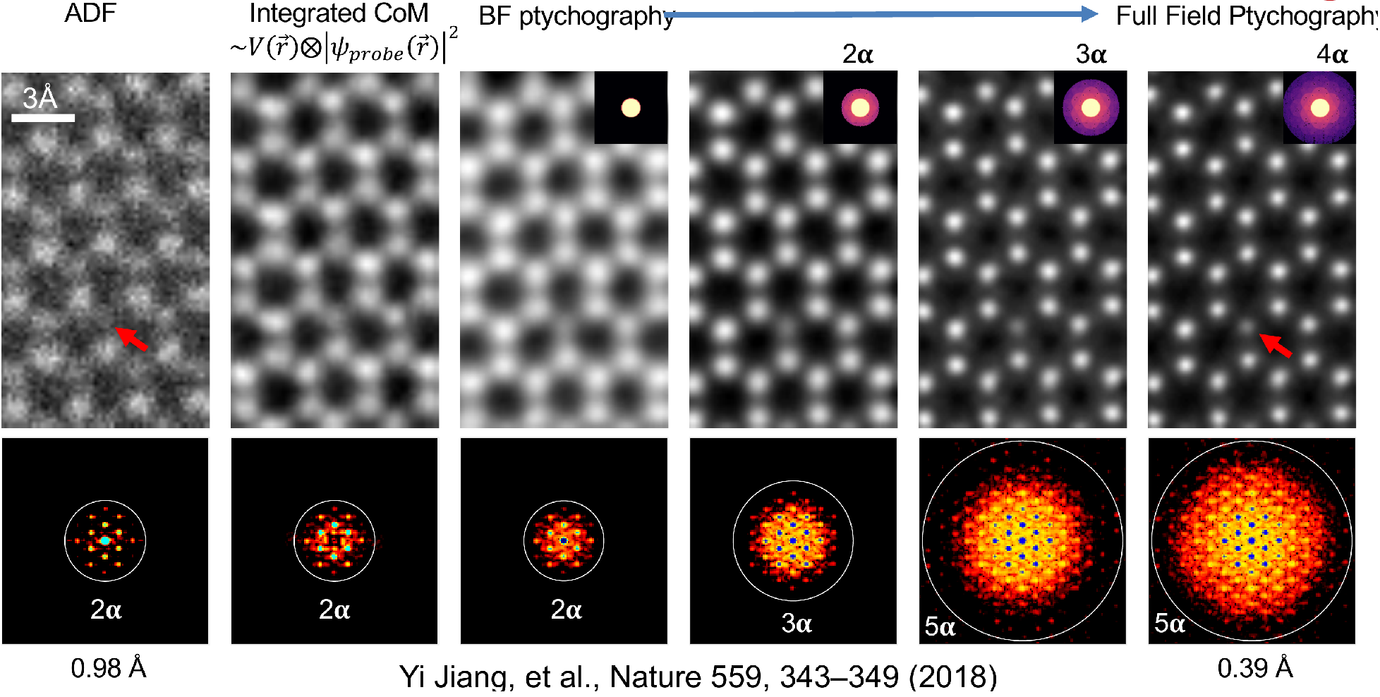
Dose vs. Resolution: 2 Regimes

[1]

Low Dose Regime

• Poisson noise uncertainty >> probe size
• Resolution scales as \(d \propto \frac{1}{\sqrt{N}}\)
• Ptychography provides 2x information limit compared to ADF at same dose

High Dose Regime

• Probe size limited by diffraction
• ADF resolution saturates
• Ptychographic resolution continues improving with dose (2-3x better)

[1] Chen, Zhen et al. (2020), doi:10.1038/s41467-020-16688-6, slide credit: D. Muller, M&M PMC 2023

Key parameters for experimental data: scan step size

[1]

[1] Skoupy, R et al. (2025), doi:10.1038/s41598-025-09871-6

Key parameters for experimental data: detector sampling

[1]

[1] Skoupy, R et al. (2025), doi:10.1038/s41598-025-09871-6

The Strong Phase Approximation (SPA)

The Strong Phase Approximation (SPA) models the interaction between the electron beam and specimen as a simple phase shift:

\[\psi(r) = \psi_0(r) e^{i\sigma V(r)}\]

where:

• \(\psi(r)\) is the exit wave
• \(\psi_0(r)\) is the incident wave

• \(\sigma\) is the interaction parameter (depends on beam energy)
• \(V(r)\) is the specimen projected potential

Key assumptions:

• Probe shape remains unchanged: \(|\psi(r)|^2 = |\psi_0(r)|^2\)
• Neglects beam spreading and propagation effects
• Treats specimen potential as a pure phase object

Limitations

The SPA breaks down for:

• Thick specimens (>10-20 nm)
• Low energy electrons (<60 keV)
• Strong scattering potentials

Multi-slice ptychography for thick samples

[1]

• High resolution preserved up to at least 30 nm thick sample
• Phase change is linearly dependent on thickness

Ambiguity in depth sectioning: The Missing Wedge

• probe propagator in multi-slice ptychography has a characteristic form:

\[\mathbb{P}(\mathbf{k}, \Delta z) = \exp(-i\pi \lambda \Delta z|\mathbf{k}_r|^2)\]

• leads to lines of constant phase where:

\[\Delta z \propto \frac{1}{|\mathbf{k}_r|^2}\]

• This relationship creates an ambiguity in depth sectioning, known as the “missing wedge” problem.

• To address this, regularization is applied to the object layers using:

\[W(\mathbf{k}) = 1 - \arctan\left(\frac{\beta^2 k_z^2}{k_r^2}\right)/(\pi/2)\]

[1]

where:

• \(\beta\) is the weighting strength parameter
• \(k_z\) is the wave vector component along the optical axis
• \(k_r\) is the transverse wave vector magnitude

This regularization helps stabilize the reconstruction while preserving high-frequency information.

[1] Chen, Zhen et al. (2021), doi:10.1126/science.abg2533, slide credit: D. Muller, M&M PMC 2023

Thermal Vibrations as a Resolution Limit: MS-Ptycho of PrScO3

[1]

• Thermal vibrations limit resolution
• Resolution limit of 22pm

[1] Chen, Zhen et al. (2021), doi:10.1126/science.abg2533

Implementing ptychography with gradient descent: the cropping operation

#| classes: "tall-cell"

import torch

def crop_windows(image, positions, window_size):
    """
    Crop windows from an image at specified positions using PyTorch.
    Windows are cropped starting from the top-left corner of the specified position.
    Positions wrap around image boundaries.
    
    Args:
        image (torch.Tensor): Input image tensor
        positions (torch.Tensor): Kx2 tensor of (x,y) positions
        window_size (int): Size of square window to crop
        
    Returns:
        torch.Tensor: Tensor of K cropped windows
    """
    # Initialize output tensor
    num_windows = positions.shape[0]
    windows = []
    h, w = image.shape
    
    # Crop window at each position
    for i, (x, y) in enumerate(positions):
        # Get wrapped indices
        x_indices = torch.arange(x, x + window_size) % w
        y_indices = torch.arange(y, y + window_size) % h
        
        # Create meshgrid of indices
        Y, X = torch.meshgrid(y_indices, x_indices, indexing='ij')
        
        # Index image with wrapped coordinates
        window = image[Y, X]
        windows.append(window)
        
    windows = torch.stack(windows, dim=0)
    return windows

Implementing ptychography with gradient descent: the forward model

#| classes: "tall-cell"

def forward_model(probe, object_func, positions, window_size):
    """
    Implement the ptychographic forward model using PyTorch.
    
    Args:
        probe (torch.Tensor): Complex probe function
        object_func (torch.Tensor): Complex object function 
        positions (torch.Tensor): Kx2 tensor of (x,y) scan positions
        window_size (int): Size of square window to crop
        
    Returns:
        torch.Tensor: Stack of K diffraction patterns
    """
    # Crop object windows at scan positions
    object_windows = crop_windows(object_func, positions, window_size)
    
    # Multiply probe with object windows
    exit_waves = probe * object_windows
    
    # Take Fourier transform
    diffraction = torch.fft.fft2(exit_waves)
    
    # Calculate intensity (magnitude squared)
    intensity = torch.abs(diffraction) 
    
    return intensity

Implementing ptychography with gradient descent: generating simulated data 1

#| fig-height: 4
#| fig-width: 10
#| code-fold: true
#| code-summary: "Show the code"

import numpy as np
import torch as th 
import skimage.data as skdata  
import skimage.transform as sktrans
import matplotlib.pyplot as plt
from scipy.ndimage import gaussian_filter
# Create defocused wave function
def defocused_wave(size=32):
 
    x = th.linspace(-1, 1, size)
    y = th.linspace(-1, 1, size)
    X, Y = th.meshgrid(x, y, indexing='ij')
    R = th.sqrt(X**2 + Y**2)
    
    # Phase function simulating defocus
    k = 8  # Wave number
    z = 0.1 # Defocus distance
    phase = k * (R**2)/(2*z)

    # Create circular amplitude mask
    center = size // 2
    Y, X = th.meshgrid(th.arange(size), th.arange(size))
    dist_from_center = th.sqrt((X - center)**2 + (Y - center)**2)
    radius = size // 4  # Adjust radius as needed
    amplitude_mask = (dist_from_center <= radius).float()
 
    # Complex wave function
    wave = amplitude_mask.to(th.float32) * th.exp(1j * phase)
    wave = th.fft.fftshift(wave)
    wave = th.fft.ifft2(wave)
    wave = th.fft.fftshift(wave)
    
    return wave
# Define PSNR function
def PSNR(img1, img2):
    """
    Calculate Peak Signal-to-Noise Ratio between two images
    
    Args:
        img1, img2: numpy arrays of same shape
        
    Returns:
        PSNR value in dB
    """
    mse = np.mean((img1 - img2) ** 2)
    if mse == 0:
        return float('inf')
    max_pixel = 1.0  # assuming normalized images [0,1]
    return 20 * np.log10(max_pixel / np.sqrt(mse))

# Define SSIM function
def SSIM(img1, img2):
    """
    Calculate Structural Similarity Index between two images
    
    Args:
        img1, img2: numpy arrays of same shape
        
    Returns:
        SSIM value between -1 and 1 (1 = identical images)
    """
    from skimage.metrics import structural_similarity as ssim
    return ssim(img1, img2, data_range=1.0)


img = skdata.astronaut()

img = sktrans.resize(img, (64, 64))
img = gaussian_filter(img, sigma=1)
# Convert to grayscale by taking mean across color channels
img = np.mean(img, axis=2)
img = img.astype(np.float32) / 255.0
img = th.from_numpy(img)  

Implementing ptychography with gradient descent: generating simulated data 2

# Generate and display the wave function
wave = defocused_wave(size=64)
wave = wave / th.norm(wave)
fig, (ax1, ax2) = plt.subplots(1, 2, figsize=(10, 4))
ax1.imshow(th.abs(wave), cmap='gray')
ax1.set_title('Amplitude')
ax1.axis('off')
# Plot phase
ax2.imshow(th.angle(wave), cmap='hsv')
ax2.set_title('Phase')
ax2.axis('off')
plt.tight_layout()
plt.show()

Implementing ptychography with gradient descent: generating simulated data 3

# Create 2D grid of positions with step size 4
x = th.arange(-16, 64-16, 4)
y = th.arange(-16, 64-16, 4) 
    
X, Y = th.meshgrid(x, y, indexing='ij')
positions = th.stack([X.flatten(), Y.flatten()], dim=1)

# Plot image with scan positions overlaid
plt.figure(figsize=(6,6))
plt.imshow(img.numpy(), cmap='gray')
plt.scatter(positions[:,0], positions[:,1], c='red', alpha=0.5, s=20)
plt.title('Scan positions overlaid on image')
plt.axis('off')
plt.show()

Implementing ptychography with gradient descent: generating simulated data 4

complex_image = torch.polar(th.ones_like(img), img/img.max()*0.4)
measured_amplitude = forward_model(wave, complex_image, positions, wave.shape[0]) + 1e-10

# Plot intensities as a mosaic
n = int(np.sqrt(len(positions)))  # Grid size
from torchvision.utils import make_grid

# Reshape and normalize the measured amplitudes for visualization
grid_images = torch.fft.fftshift(measured_amplitude[:n*n])  # Take only complete grid
grid_images = grid_images / grid_images.max()  # Normalize to [0,1]

# Create image grid
grid = make_grid(grid_images.unsqueeze(1), nrow=n, padding=2, normalize=False)
# Permute dimensions to get correct shape (H,W,C)
grid = grid.permute(1, 2, 0)

# Display the grid
plt.figure(figsize=(12, 12))
plt.imshow(grid.squeeze().numpy(), cmap='gray')
plt.title('Intensity patterns at each scan position')
plt.axis('off')
plt.show()

Implementing ptychography with gradient descent: solving the inverse problem

#| code-fold: true
#| code-summary: "Show the code"

# Initialize random guess for object
guess = th.polar(th.ones_like(img), th.randn_like(img)*1e-8)
guess.requires_grad = True
# Optimization parameters
num_epochs = 20
batch_size = len(positions) // 2
learning_rate = 3e-2
optimizer = th.optim.Adam([guess], lr=learning_rate)
print(len(positions))
# Training loop
for epoch in range(num_epochs):
    # Randomly select batch_size positions
    batch_indices = th.randperm(len(positions))

    losses = 0

    # Process batch_size positions at a time
    for i in range(0, len(positions), batch_size):
        # print(batch_indices[i:i+batch_size])
        batch_pos = positions[batch_indices[i:i+batch_size]]  # Get batch of positions
        batch_amp = measured_amplitude[batch_indices[i:i+batch_size]]  # Get corresponding intensities
        
        # Forward pass for this position
        pred_amp = forward_model(wave, guess, batch_pos, wave.shape[0])
        
        # Calculate loss for this position
        loss = torch.nn.functional.mse_loss(pred_amp, batch_amp)

        losses += loss.item()
        
        # Backward pass
        optimizer.zero_grad()
        loss.backward()
        optimizer.step()
    
    # Print progress every 10 epochs
    if (epoch + 1) % 1 == 0:
        print(f'Epoch [{epoch+1}/{num_epochs}], Loss: {losses:.4f}')

# Plot results
fig, (ax1, ax2, ax3) = plt.subplots(1, 3, figsize=(15, 5))

gt_phase = th.angle(complex_image)
gt_phase -= gt_phase.min()

res_phase = th.angle(guess).detach().numpy()
res_phase -= res_phase.min()

# Plot original phase
ax1.imshow(gt_phase, cmap='gray', vmax=gt_phase.max(), vmin=gt_phase.min())
ax1.set_title('Original Phase')
ax1.axis('off')

# Plot reconstructed phase
ax2.imshow(res_phase, cmap='gray', vmax=gt_phase.max(), vmin=gt_phase.min())
ax2.set_title('Reconstructed Phase')
ax2.axis('off')

# Plot absolute error
error = th.abs(th.angle(guess).detach() - th.angle(complex_image))
ax3.imshow(error.numpy(), cmap='hot')
ax3.set_title('Absolute Error')
ax3.axis('off')

plt.tight_layout()
plt.show()
 

Ptychographic Tomography Solves Nanostructures

Note

First 3D atomic structure solved with phase-contrast tomography.
Novel ZrTe₂ phase, confirmed stable with DFT simulations.

Pelz, Philipp M. et al. (2023), doi:10.1038/s41467-023-43634-z

Depth Resolution Progress Over Time

2022: 2.2 Å in 9nm thick volume using SSPT

2023: 2.0 Å in 18nm thick volume using MSPT

2024: 0.8 Å in 11nm thick volume using E2E-MSPT

Pelz, Philipp M. et al. (2023), doi:10.1038/s41467-023-43634-z, Romanov, Andrey et al. (2024), doi:10.1088/2515-7639/ad9ad2, You, Shengbo et al. (2024), doi:10.1088/1402-4896/ad9a1a

Multi-Slice Ptychographic Tomography

Perform MSP reconstruction
for each tilt angle
and project the potential along z







✅ Advantages:
- Decouple tomographic alignment from ptychographic reconstruction
- Can use positions and alignment as input to E2E-MSPT

Multi-slice Ptychographic Tomography forward model

❌ Disadvantage:
- Loses some 3D info from MSP

Romanov, Andrey et al. (2024), doi:10.1088/2515-7639/ad9ad2

Joint Tomography and Rigid Alignment enables atomic resolution of beyond-DOF volumes

Note

Enabled by reaching sub-pixel alignment at each scale

Romanov, Andrey et al. (2024), doi:10.1088/2515-7639/ad9ad2

3x DOF volumes display atomic resolution

Note

Volume size: (18.2 nm)³ Voxel size: 0.3 Å

Romanov, Andrey et al. (2024), doi:10.1088/2515-7639/ad9ad2

Orthoslices reveal lattice in all 3 dimensions

scale: 1 nm

Note

Lattice resolved, but Co atom contrast overpower O contrast
=> Around 1 Å z resolution required to resolve O atoms

Romanov, Andrey et al. (2024), doi:10.1088/2515-7639/ad9ad2

End-to-end reconstruction - putting all pieces together

Fully E2E-MSPT reconstruction includes

1. affine resampling of potential volume
   
2. z-resampling of potential volume (save compute)
   
3. batch-croppping and mixed-state multi-slice model
   
4. far-field propagation
   
5. gradient backpropagation through full model

Note

The most accurate approximation for 4D-STEM tomography to-date

You, Shengbo et al. (2024), doi:10.1088/1402-4896/ad9a1a

Successive approximations help initialize “nuisance parameters”

Note

Successive initialization reduces compute
overhead of the most accurate models

You, Shengbo et al. (2024), doi:10.1088/1402-4896/ad9a1a

Limited-Angle Tomography is an option now

Note

Light and heavy atoms recovered in 3D with 90-degree tilt range.

You, Shengbo et al. (2024), doi:10.1088/1402-4896/ad9a1a

Sub-Ångstrom alignment accuracy demonstrated in simulations

Frozen phonon 4D-STEM simulation
Al₂O₃ nanoparticle

Phase projections at different tilt angles

Alignment accuracy

Note

Mean alignment error < voxel size (0.4 Å)

You, Shengbo et al. (2024), doi:10.1088/1402-4896/ad9a1a

Volume displays clear atomic contrast in 3D

Note

Recovery of missing wedge with only physical priors.
Reached Nyquist resolution of 0.82 Å

You, Shengbo et al. (2024), doi:10.1088/1402-4896/ad9a1a

Volume displays clear atomic contrast in 3D

2

1

Note

All directions recovered well

Dose reduction by sub-sampling

Note

2.8 Å resolution with 2.2*10⁴ e^-/Ų - virtual sub-sampling
0.82 Å resolution with 12x sub-sampling

You, Shengbo et al. (2024), doi:10.1088/1402-4896/ad9a1a

Wiring up your microscope for automated 4D-STEM tomography

Note

SerialEM plugins allow custom detectors and online image processing

Also with SerialEM plugin: Seifer, Shahar et al. (2024), doi:10.1093/mam/ozae050

Adopting the cryo-EM playbook: PACE-Tomo SOTA

Tracking taret on tilt-axis Imaging target off tilt-axis

Geometric sample model that tracks shifts in 3D

Multi-target acquisition

+- 50nm tracking errors

Note

Cryo-EM automation tools have nearly all desired features
but lack tracking precision and can be enhanced by real-time 4D-STEM

Eisenstein, Fabian et al. (2023), doi:10.1038/s41592-022-01690-1

Automated 4D-STEM tomography: first target

Sample synthesized by Xingchen Ye Group:
Gd₂O₃ nanohelices

Liu, Yang et al. (2020), doi:10.1021/jacs.0c05175

Automated 4D-STEM tomography at atomic resolution

• Timing: 2 min. per tilt, 90 min. per tilt series
  
• No human intervention required after target selection

Bla

Note

Cryo-EM automation tools can be adapted and enhanced for automated atomic resolution 4D-STEM tomography

You, Pelz et al. in preparation

References

Solving complex nanostructures with ptychographic atomic electron tomography, Nature Communications, Philipp M Pelz, Sinéad M Griffin, Scott Stonemeyer, & others https://doi.org/10.1038/s41467-023-43634-z.

An improved ptychographical phase retrieval algorithm for diffractive imaging, Ultramicroscopy, Andrew M Maiden & John M Rodenburg https://doi.org/10.1016/j.ultramic.2009.05.012.

Probe retrieval in ptychographic coherent diffractive imaging, Nature, Pierre Thibault & Andreas Menzel https://doi.org/10.1038/nature11806.

Ptychographic coherent diffractive imaging with orthogonal probe relaxation, Optics Express, Michal Odstrcil, Mirko Holler, & Manuel Guizar-Sicairos https://doi.org/10.1364/OE.24.008360.

Mixed-state electron ptychography enables sub-nanometer resolution imaging with simultaneous denoising, Nature Communications, Zhen Chen, Yi Jiang, Yu-Tsun Shao, Megan E Holtz, Michal Odstrčil, Manuel Guizar-Sicairos, Ingo Hanke, Steffen Ganschow, Darrell G Schlom, & David A Muller https://doi.org/10.1038/s41467-020-16688-6.

Ptychoscopy: A user friendly experimental design tool for ptychography, Scientific Reports, R Skoupy, E Müller, TJ Pennycook, & others https://doi.org/10.1038/s41598-025-09871-6.

Electron ptychography achieves atomic-resolution limits set by lattice vibrations, Science, Zhen Chen, Michal Odstrcil, Yi Jiang, Yimo Han, Ming-Hu Chiu, Lain-Jong Li, & David A Muller https://doi.org/10.1126/science.abg2533.

Solving complex nanostructures with ptychographic atomic electron tomography, Nature Communications, Philipp M. Pelz, Sinéad M. Griffin, Scott Stonemeyer, Derek Popple, Hannah DeVyldere, Peter Ercius, Alex Zettl, Mary C. Scott, & Colin Ophus https://doi.org/10.1038/s41467-023-43634-z.

Multi-slice electron ptychographic tomography for three-dimensional phase-contrast microscopy beyond the depth of focus limits, Journal of Physics: Materials, Andrey Romanov, Min Gee Cho, Mary Cooper Scott, & Philipp Pelz https://doi.org/10.1088/2515-7639/ad9ad2.

Near-isotropic sub-ångstrom 3d resolution phase contrast imaging achieved by end-to-end ptychographic electron tomography, Physica Scripta, Shengbo You, Andrey Romanov, & Philipp M Pelz https://doi.org/10.1088/1402-4896/ad9a1a.