Data Science for Electron Microscopy
Week 11: Uncertainty, Gaussian processes & autonomous EM

Prof. Dr. Philipp Pelz

FAU Erlangen-Nürnberg

Institute of Micro- and Nanostructure Research

Recap: Week 10 and today’s question

• Week 10: attention, transformers and graph networks — the last architecture family of the course. CNN = grid graph, GNN = sparse graph, transformer = fully connected graph. We read attention maps and learned that attention ≠ explanation.
• The gap every architecture shares: a ViT, a GNN or a U-Net outputs a softmax or a number — always, with the same apparent confidence, whether the input looks like the training data or not.
• Today’s question: how sure is the model, and what should we do with that information? Can we trust this prediction? Where should the microscope measure next?
• Today’s answer, in three steps: (1) quantify uncertainty (ensembles, MC dropout, GPs), (2) certify it (calibration, conformal prediction, OOD gate), (3) act on it (Bayesian optimisation, deep kernel learning, autonomous 4D-STEM).

• Open from Week 10: “last week we asked where the transformer looked. Today we ask how sure it is — and whether that number means anything.” Attention maps were explainability for a model family; uncertainty is the trust signal that works for every family.
• This lecture merges what used to be two weeks (uncertainty & GPs, and active/automated EM). The unifying sentence: “an honest error bar is both a trust gate and a steering signal.”
• EM anchor: a phase-boundary pixel in an Fe–O EELS map. The segmentation network says “Fe₂O₃”. With what probability? And if it does not know — should we measure there again?
• Pacing: 3 minutes. Key phrase to land: “a number without an error bar is not a deliverable.”
• Transition: “Here is the road map.”

Road map, learning outcomes and self-study

Road map (≈ 90 min)

1. Why point predictions are dangerous · aleatoric vs epistemic
2. Uncertainty for deep nets: ensembles, MC dropout, reject threshold
3. Are the error bars honest? calibration, ECE, conformal & CQR
4. Gaussian processes: prior, posterior, kernels
5. Acting on uncertainty: Bayesian optimisation
6. Deep kernel learning & automated 4D-STEM
7. OOD detection as a trust gate · RL / agents outlook

After today you can

• separate aleatoric from epistemic uncertainty and name a method for each
• read a reliability diagram, compute ECE, build a split-conformal interval
• write down and interpret the two GP posterior formulas
• run a BO loop and choose an acquisition function
• design a trust gate (σ + OOD score) for a deployed EM model

Self-study: notebooks/week11_gp_bo.ipynb (GP → conformal → BO, CPU, < 2 min)

• One minute. Gesture at the structure: quantify → certify → act → guard.
• Timing plan (90 min, ~5 min slack):
  • 0–4: recap + road map
  • 4–14: why uncertainty · aleatoric vs epistemic · predictive distribution / law of total variance
  • 14–22: ensembles, MC dropout, MetalDAM case study, reject-for-review
  • 22–32: calibration + ECE + temperature scaling · split conformal, CQR · who-guarantees-what table
  • 32–46: GPs — definition, prior → posterior, the two formulas, balloon, length-scale, marginal likelihood, scorecard
  • 46–57: BO — explore/exploit, experiment design, loop, acquisition functions, snapshots, BO vs random
  • 57–64: DKL + automated 4D-STEM + choosing the tool
  • 64–73: OOD trust gate (3 slides) · RL / agents outlook
  • 73–84: notebook, key results, summary, must-know, Week 12 teaser
  • 84–90: slack / questions (backup slides: GP σ-map, acquisition-function comparison)
• The learning outcomes are the exam targets. The two GP formulas and the split-conformal recipe are the two “write it down from memory” items.
• The notebook has three parts matching the lecture: Part A GP regression, Part B split conformal & CQR, Part C BO loop. Recommend students do Part A before next week’s lecture at the latest.
• Transition: “Why do we even need error bars?”

Why a point prediction is dangerous for EM decisions

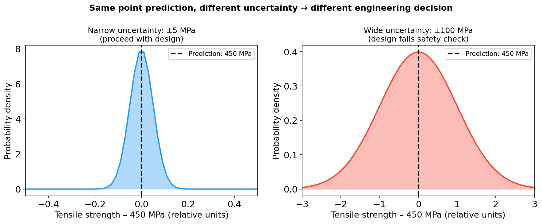
Two predictive distributions with the same point prediction (450 MPa) but radically different uncertainty. Left: ±5 MPa — the part passes the safety factor. Right: ±100 MPa — the design must be rejected. The decision lives in the band, not in the mean.

• Same mean, same label, opposite decision. The left model is a yes; the right is a no. The mean alone cannot distinguish them.
• Engineering and lab decisions are threshold decisions: accept/reject a segmentation, release/retest a part, measure here or not. A threshold needs a distribution, not a number (ML-PC U12 framing).
• EM anchor: a GP predicting Fe³⁺ fraction at a new composition. ±0.02 → informative. ±0.40 → “I have no idea — measure before deciding.”
• Write on the board: “an overconfident model is more dangerous than an inaccurate one.”

When point predictions fail in electron microscopy

• Phase identification: “Fe₂O₃” at a boundary pixel — clean decision or coin-flip?
• Extrapolation without warning: trained on 200–500 °C, predicts 600 °C with the same confidence Bishop, Christopher M., (2006).
• New instrument or session: detector swap → confident, smooth-looking, wrong maps. Errors are silent.
• Expensive experiment design: honest error bars tell you what is worth measuring.
• Root cause: empirical-risk minimisation gives the model no incentive to express ignorance.

• Examples in full: a CNN labels a boundary pixel “Fe₂O₃” and misidentifications propagate silently into phase maps; a model trained on 200–500 °C specimens does not know it is extrapolating at 600 °C; a net trained on SEM #1 runs on SEM #2 after a detector swap; 8 h of instrument time on a composition you already know well is wasted.
• ERM rewards average accuracy on the training distribution — nothing more.
• “Silent failure” is the key phrase: a model that returns NaN is safe — you know it failed. A model that returns a confident wrong number is the dangerous one.
• The ERM point links back to Week 4: MSE/cross-entropy measure accuracy, not calibration. A model can have great test MSE and terrible practical safety.
• The four bullets map to today’s four tools: classification confidence (ensembles/MC dropout), extrapolation (GP variance, OOD), instrument shift (calibration, OOD gate), experiment design (BO).
• Transition: “To fix this we need to be precise about what kind of uncertainty we mean.”

Aleatoric vs epistemic uncertainty

• Aleatoric (alea = dice): irreducible randomness in the data-generating process — shot noise, detector read noise, grain-to-grain scatter. More data of the same kind does not remove it.
• Epistemic (episteme = knowledge): uncertainty from limited knowledge — we measured 8 compositions out of infinitely many, the model never saw this microscope. It shrinks as we add (the right) data.
• Diagnostic test: “Would measuring more of the same kind of data reduce this uncertainty?” Yes → epistemic. No → aleatoric Bishop, Christopher M., (2006).
• Why it matters: aleatoric sets the achievable precision (and the right loss — Week 2); epistemic tells you where to invest the next instrument-hour and when not to trust the model.

• Run the diagnostic live with EM examples: grain-to-grain hardness scatter (aleatoric), hardness model fitted to 5 grains (epistemic), detector thermal noise (aleatoric), a model applied to a new alloy family (epistemic).
• Week 2 callback: the noise model (Poisson/Gaussian) is the aleatoric model; it decided our loss. Today we add the epistemic part.
• Subtle point for the strong students: at a hard phase boundary, class ambiguity is aleatoric (the pixel genuinely mixes phases); a class the model never saw is epistemic. Entropy of the softmax mixes both.

Aleatoric vs epistemic in EM: visual comparison

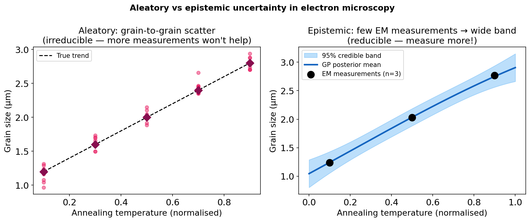
Left: aleatoric — grain-to-grain scatter in grain size at a fixed annealing temperature; more measurements reveal the distribution but do not remove the scatter. Right: epistemic — a GP fitted to 3 EELS measurements is uncertain everywhere except near the measured compositions; measuring more narrows the band.

• Left: scatter is the material’s real variability. A smaller error bar on the mean comes from averaging more grains, not from a better instrument.
• Right: the band collapses at the three measured compositions and stays wide between and beyond them.
• Ask: “which uncertainty shrinks if I measure 10 more grains at the same temperature?” (the uncertainty of the mean, not the scatter). “Which shrinks if I measure 3 more compositions?” (right panel). Get both answers.

From a point estimate to a predictive distribution

\[p(y_* \mid \mathbf{x}_*, \mathcal{D}) = \int p(y_* \mid \mathbf{x}_*, \theta)\, p(\theta \mid \mathcal{D})\, d\theta\]

\[ \underbrace{\mathrm{Var}[y_*]}_{\text{total}} = \underbrace{\mathbb{E}_{\theta}\big[\sigma_\epsilon^2(\mathbf{x}_*;\theta)\big]}_{\text{aleatoric}} + \underbrace{\mathrm{Var}_{\theta}\big[\mu(\mathbf{x}_*;\theta)\big]}_{\text{epistemic}} \]

• ERM / MSE returns one \(\hat\theta\) → one number \(\hat y\) (MSE = MLE under Gaussian noise, Week 4). Bayesian averaging over plausible \(\theta\) returns a distribution.
• Epistemic term = disagreement between plausible models. Near data they agree; away from data they disagree Murphy, Kevin P., (2012).
• Every method today approximates this integral: ensembles (M samples of \(\theta\)), MC dropout (random masks), GPs (exact, closed form).

• Read the integral as a sentence: “for every parameter vector the data finds plausible, ask what it predicts, and average weighted by plausibility.”
• The variance decomposition (law of total variance) is the formal version of the aleatoric/epistemic split. Write it on the board; underline “does not shrink” under aleatoric and “shrinks” under epistemic.
• Road-map sentence: “Deep ensembles are a crude Monte-Carlo estimate of this integral with M=5 samples. MC dropout is a cheaper one. The GP does it exactly.”
• Active-learning hook: measure where the epistemic term is largest.

Uncertainty for deep networks: ensembles and MC dropout

Deep ensembles Lakshminarayanan, Balaji et al., (2017)

• Train \(M \approx 5\) networks from different random initialisations / data orders.
• Mean of members = prediction; spread = epistemic uncertainty.
• Different local minima → genuine diversity → best empirical calibration of simple NN methods.
• Cost: \(M\times\) training, \(M\times\) inference (parallelisable).

MC dropout Gal, Yarin et al., (2016)

• Keep dropout on at inference; run \(T \approx 30\) stochastic passes.
• Interpretable as approximate variational inference with a Bernoulli posterior.
• Zero extra training cost — works on any net trained with dropout.
• Pitfall: model.eval() switches dropout off.

For classification, per pixel \(i\): \(\bar{\mathbf{p}}_i = \frac{1}{T}\sum_t \mathbf{p}_i^{(t)}\), predictive entropy \(H_i = -\sum_c \bar p_{i,c}\log \bar p_{i,c}\).

• Ensembles: the loss landscape of a deep net has many minima; different seeds land in different ones. Where data are dense they agree, where data are sparse they disagree — that disagreement is the epistemic signal, no Bayesian formalism needed.
• MC dropout: one-line change, but half of student implementations get it silently wrong by calling model.eval(). Enable dropout layers explicitly.
• Use the entropy of the mean softmax, not the variance of the softmax outputs — the entropy of \(\bar p\) is the “total uncertainty”; separating aleatoric/epistemic needs mutual information and is rarely worth it.
• \(T=30\) is a typical knee — validate on a reliability diagram rather than trusting the number.
• Rule of thumb: MC dropout if a trained network already exists and compute is tight; ensemble if calibration quality is critical.

Ensembles vs MC dropout on a 1-D regression

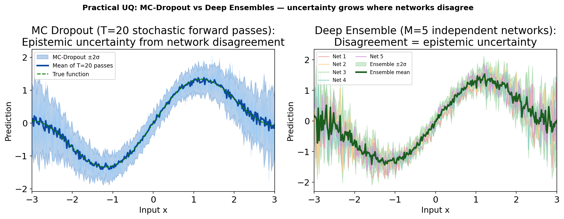
Left: MC dropout — stochastic forward passes (light blue) and mean ±2σ. Right: a deep ensemble of 5 independently trained networks (coloured) and mean ±2σ (green). Both widen away from data; ensembles are empirically better calibrated Lakshminarayanan, Balaji et al., (2017).

• Left: same weights, different masks — the variance reflects the approximate posterior; it depends on the dropout rate (too low → overconfident, too high → everything uncertain).
• Right: five entirely different training runs. Their disagreement grows in the data gap and beyond the range.
• Honest caveat: neither method is guaranteed to widen far from data — a ReLU network can extrapolate linearly and all members may agree. This is why we still need an OOD check later today.

Case study: MC dropout for SEM segmentation (MetalDAM)

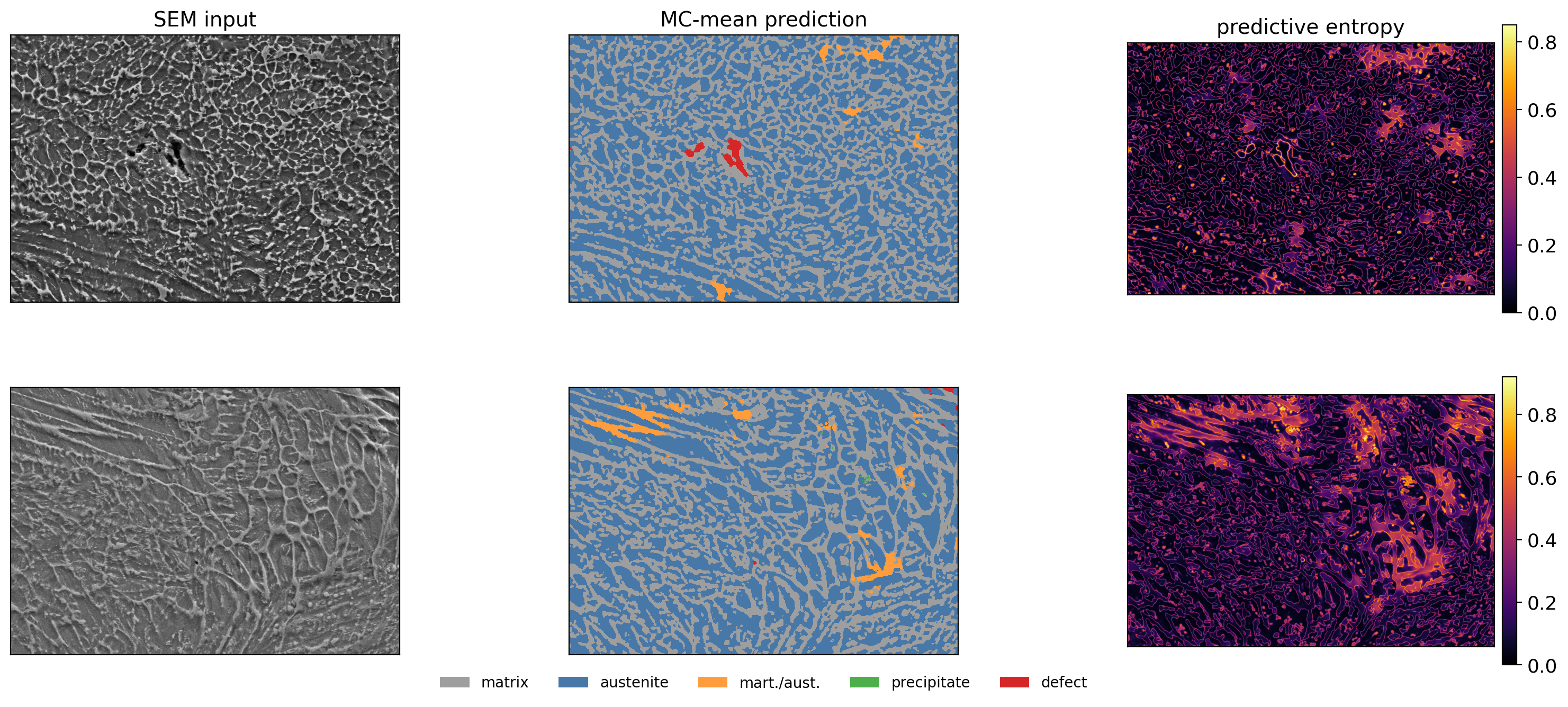
Two held-out MetalDAM micrographs of additively manufactured steel: SEM input, MC-mean prediction, per-pixel predictive entropy (\(T{=}30\)). Low entropy inside well-formed matrix/austenite regions; high entropy at phase boundaries, in ambiguous martensite/austenite laths and at defect rims. Data: MetalDAM ArcelorMittal et al., (2021); Luengo, Julián et al., (2022), doi:10.1016/j.inffus.2021.09.018; figure from ML-PC Unit 12.

• U-Net with dropout (p≈0.2) in bottleneck and decoder, trained on 42 expert-labelled micrographs; whole micrographs held out (Week 4 honest validation — split by image, not by tile).
• The uncertainty map is self-interpretable: it lights up exactly where a human expert would hesitate. If yours does not, suspect a calibration bug (dropout too low, one dropout layer only).
• Class imbalance: defect pixels are 0.7% of the data, precipitates 0.2% (mostly unannotated — label noise, Week 8 callback).
• Anti-pattern: blurring the entropy map before thresholding. Its spatial resolution is the point.

Reject-for-human-review: turning uncertainty into a decision

• Choose an entropy threshold \(\tau\): pixels with \(H_i > \tau\) go to an operator; the rest are auto-classified.
• Sweep \(\tau\) → operating curve (review rate vs defect recall). Report the curve, not one threshold.
• The operating point is a cost decision (analyst time vs missed defect), not an ML decision.
• Honest limit: the residual misses are confidently wrong — low entropy. No entropy threshold recovers them → calibration audit + OOD gate.

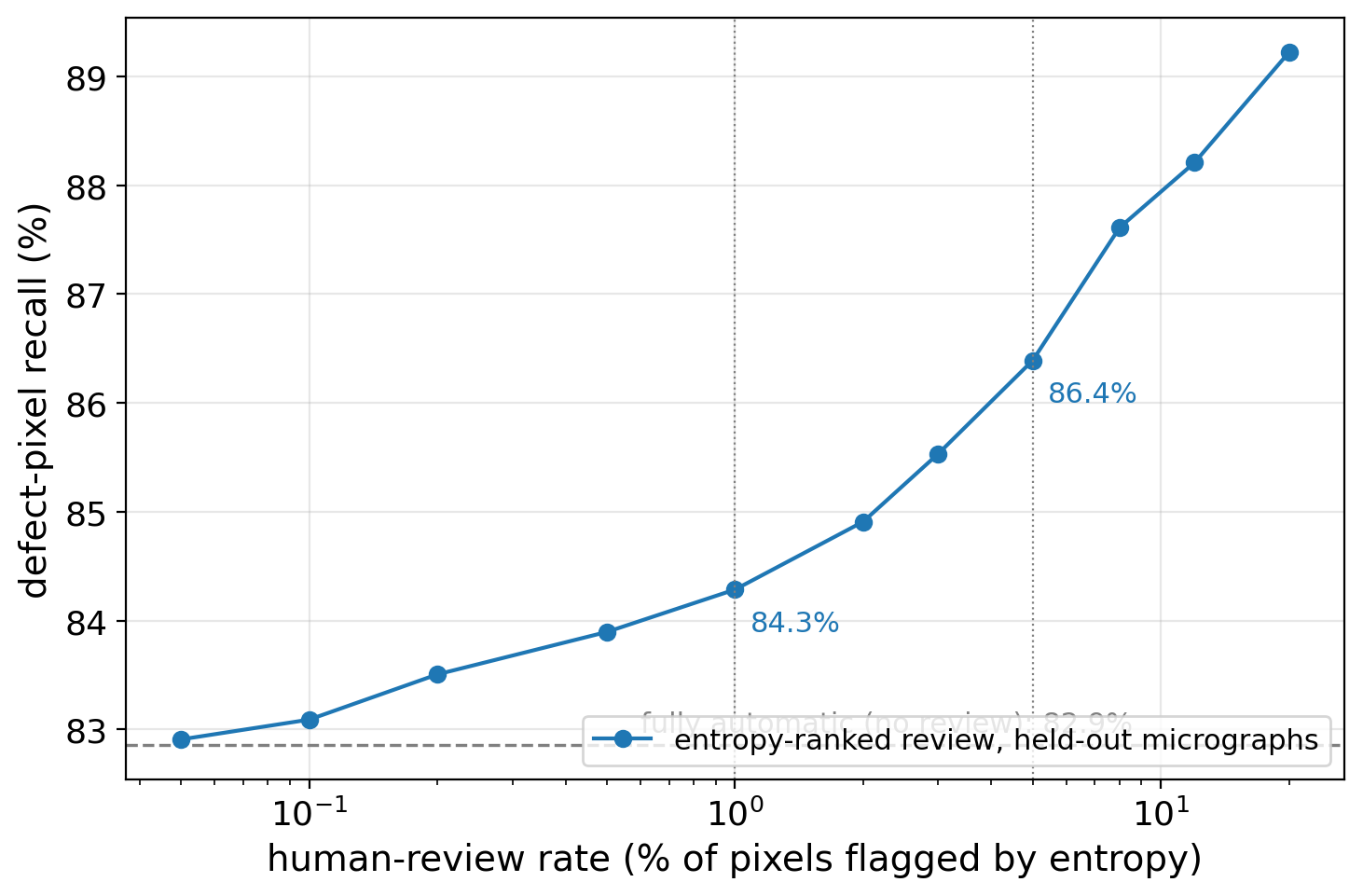
Held-out MetalDAM: fully automatic recall of defect pixels 82.9%; entropy-ranked review adds +1.4 points at 1% review and +3.5 points at 5% (ML-PC Unit 12).

• This is the practical payoff of per-pixel uncertainty: model + human in the loop. At 5% review on a 1024×703 micrograph that is ~36k pixels, clusterable into a few hundred ROIs an analyst scans in a minute.
• There is no sharp knee in this curve — say it honestly. The headline is the gap to 100%: confidently wrong pixels. That is the bridge to calibration.
• Link to Week 8 active labelling: the flagged pixels are exactly the tiles worth labelling next.
• Transition: “Are these confidences honest at all? That is calibration.”

Calibration: are the error bars honest?

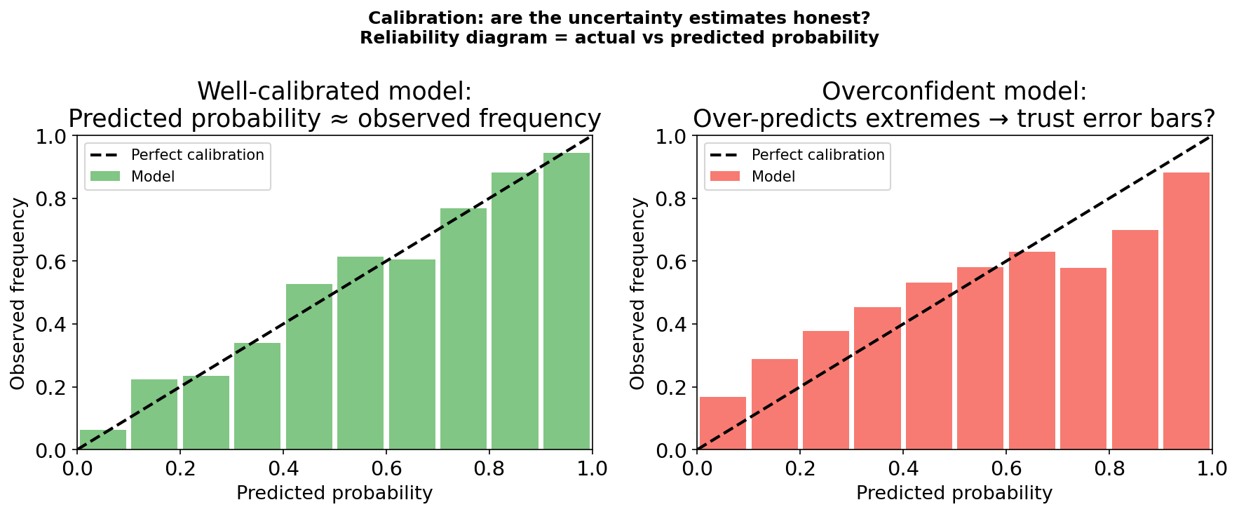
Reliability diagrams. Left: a well-calibrated classifier — predicted confidence matches observed accuracy in each bin. Right: an overconfident model — bins below the diagonal; its “90%” is right far less often than 90% of the time.

• Bin predictions by confidence (10 bins). Per bin: mean predicted confidence (x) vs observed accuracy (y). Diagonal = calibrated. Below = overconfident (dangerous), above = underconfident (wasteful but safe).
• For regression the analogue: nominal interval level vs empirical coverage.
• Modern deep nets are typically overconfident Guo, Chuan et al., (2017) — bigger, better-trained networks drift further below the diagonal.
• A GP’s 95% band is calibrated only if the kernel and noise model are right. Check it the same way.

Calibration metrics and post-hoc fixes

• Expected Calibration Error over \(B\) confidence bins: \[\mathrm{ECE} = \sum_{b=1}^{B} \frac{|\mathcal{B}_b|}{N}\,\big|\mathrm{acc}(\mathcal{B}_b) - \mathrm{conf}(\mathcal{B}_b)\big|\] 0 = perfect; always show the diagram too — the shape carries the diagnosis.
• Temperature scaling Guo, Chuan et al., (2017): \(\hat{\mathbf{p}} = \mathrm{softmax}(\mathbf{z}/T)\), one scalar \(T\) fitted on a calibration set. Changes confidences, not the argmax — accuracy is unchanged.
• The calibration set must be held out and lab-realistic: same microscope, protocol and settings as deployment, no specimen shared with training (Week 4 leakage rules apply).
• Tool shift breaks calibration: MetalDAM with a simulated detector change — ECE 9.2% → 3.5% after temperature scaling on the new tool; pixel accuracy unchanged (ML-PC U12).

• ECE is a one-number summary; bin-count choices change it. Report it with the diagram.
• Temperature scaling: one parameter, post-hoc, no retraining. It fixes global over/underconfidence; it cannot fix wrong predictions.
• Trigger list for re-calibration: detector swap, gun replacement, coating change, large chamber vent. “My accuracy dropped after the chamber vent” is a calibration failure as often as a model failure — diagnose with a reliability diagram before retraining.
• War story (ML-PC): a pore-detection pipeline dropped 96%→78% after a chamber clean; two weeks of retraining. The real bug: the contrast shift broke calibration, so a fixed confidence threshold discarded true detections. Temperature scaling on 30 images fixed the thresholding step in an hour.

Split conformal prediction: a guarantee without trusting the model

1. Split data: train / calibration (never used for fitting) / test.
2. Fit any predictor \(\hat f\) on train (GP, random forest, U-Net …).
3. Scores on calibration: \(s_i = |y_i - \hat f(\mathbf{x}_i)|\), \(i=1,\dots,n\).
4. \(\hat q\) = the \(\lceil (n+1)(1-\alpha)\rceil\)-th smallest score.
5. Output \(C(\mathbf{x}_*) = [\hat f(\mathbf{x}_*) - \hat q,\ \hat f(\mathbf{x}_*) + \hat q]\).

• Guarantee Angelopoulos, Anastasios N. et al., (2023): \(\Pr\big(y_* \in C(\mathbf{x}_*)\big) \ge 1-\alpha\) for any predictor and any distribution — provided calibration and test data are exchangeable.
• Classification: same recipe with score \(1-\hat p_{y}(\mathbf{x})\) → prediction sets (“Fe₂O₃ or FeO”) that contain the true class with prob. \(\ge 1-\alpha\).

• “Any predictor” is the selling point: no Gaussian assumption, no correct kernel. It is a wrapper.
• The \((n+1)\) correction makes the finite-sample guarantee exact; with small \(n\) the band is slightly conservative, never undercovering.
• Most common mistake: computing \(\hat q\) from training residuals. The model fits its training data too well → too narrow → undercoverage (notebook: 0.78 instead of 0.90).
• Exchangeability is the one assumption. Discovery campaigns and new microscopes violate it by design — keep this in mind for the OOD section.
• Prediction sets for classification: a set of size 1 is a confident call; size 3 means “ambiguous — look at it.”

Split conformal vs CQR on heteroscedastic EM data

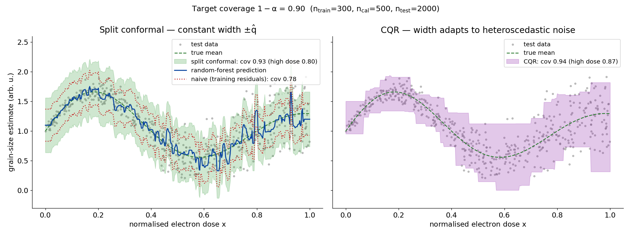
Grain-size estimate vs electron dose with noise growing with dose. Left: a random forest wrapped with split conformal — target coverage 0.90 reached (0.93) with a constant band; the naive training-residual band covers only 0.78. Right: conformalized quantile regression — same guarantee (0.94) with a band that widens with dose. Notebook Part B, SEED=42.

• Left: the guarantee holds marginally — averaged over all doses. At high dose only, split conformal covers just 0.80: too narrow where noise is large, too wide where it is small.
• Right: CQR Romano, Yaniv et al., (2019) fits lower/upper quantile regressors (\(\alpha/2\), \(1-\alpha/2\)), then conformalises them with the score \(s_i=\max(\hat q_{lo}(\mathbf{x}_i)-y_i,\ y_i-\hat q_{hi}(\mathbf{x}_i))\) and outputs \([\hat q_{lo}-\hat q,\ \hat q_{hi}+\hat q]\). High-dose coverage improves to 0.87 and the band is 2.3× wider at high dose than at low dose.
• Neither method gives conditional coverage in general — that is impossible distribution-free — but CQR gets much closer when noise is heteroscedastic.
• All numbers come from the notebook; students reproduce them in Part B.

GP bands, conformal intervals, OOD: who guarantees what?

	GP credible band	Split conformal / CQR	Needs in addition
Guarantee	only if kernel + noise model correct	finite-sample, distribution-free, marginal	—
Width	varies with distance to data	constant (split) / adaptive (CQR)	—
Holds under shift?	no — kernel may miss the shift	no — exchangeability broken	OOD gate
Steers acquisition?	yes (σ is an exploration signal)	not directly	—
Cost	\(O(N^3)\)	sort residuals	—

Rule of thumb: GP / ensembles to explore; conformal to certify in-distribution; an OOD score to decide whether you are in-distribution at all.

• This table is the spine of the second half. Conformal answers “how wide should the interval be, given we are in-distribution?” The OOD gate answers “are we in-distribution?” Neither replaces the other.
• Notebook exercise B3: evaluate the calibrated interval on dose 1.0–1.3 (never seen) → coverage drops from 0.93 to 0.70. The guarantee silently evaporates.
• MG U14 framing: conformal is ideal as a screening filter (cut 10⁵ candidates to 10³ with certified intervals), GPs for the acquisition that follows.
• Transition: “Now the model that gives honest, input-dependent uncertainty in closed form: the Gaussian process.”

Gaussian processes: a distribution over functions

• A GP is a probability distribution over functions: any finite set of values \([f(\mathbf{x}_1),\dots,f(\mathbf{x}_N)]\) is jointly Gaussian. \[f \sim \mathcal{GP}\big(m(\mathbf{x}),\ k(\mathbf{x},\mathbf{x}')\big)\]
• Fully specified by a mean function \(m(\mathbf{x})\) (usually 0 after centring) and a kernel \(k(\mathbf{x},\mathbf{x}') = \mathrm{Cov}[f(\mathbf{x}), f(\mathbf{x}')]\).
• RBF kernel: \(k(\mathbf{x},\mathbf{x}') = \sigma_f^2 \exp\!\big(-\|\mathbf{x}-\mathbf{x}'\|^2 / 2\ell^2\big)\) — nearby inputs have correlated outputs; length-scale \(\ell\) sets the correlation range, \(\sigma_f^2\) the vertical amplitude Rasmussen, Carl Edward et al., (2006).
• The kernel is the modelling decision: it encodes “compositions closer than \(\ell\) have similar Fe³⁺ fractions” — domain knowledge as a covariance.

• Concrete picture: a 2-D Gaussian gives an ellipse of likely \((x,y)\) pairs; a GP gives a cloud of likely curves. We never handle the infinite object — only its finite marginals at the inputs we care about.
• Kernel ↔︎ inductive bias (course thread): CNN = translation equivariance, GNN = permutation invariance, GP kernel = smoothness/correlation structure.
• RBF gives infinitely smooth functions; Matérn-5/2 allows kinks and is often a better default for materials properties.
• At \(|x-x'| = \ell\) the kernel is \(e^{-0.5}\approx0.6\); at \(3\ell\) it is \(\approx0.01\) — nearly independent.

Conditioning on data: prior → posterior

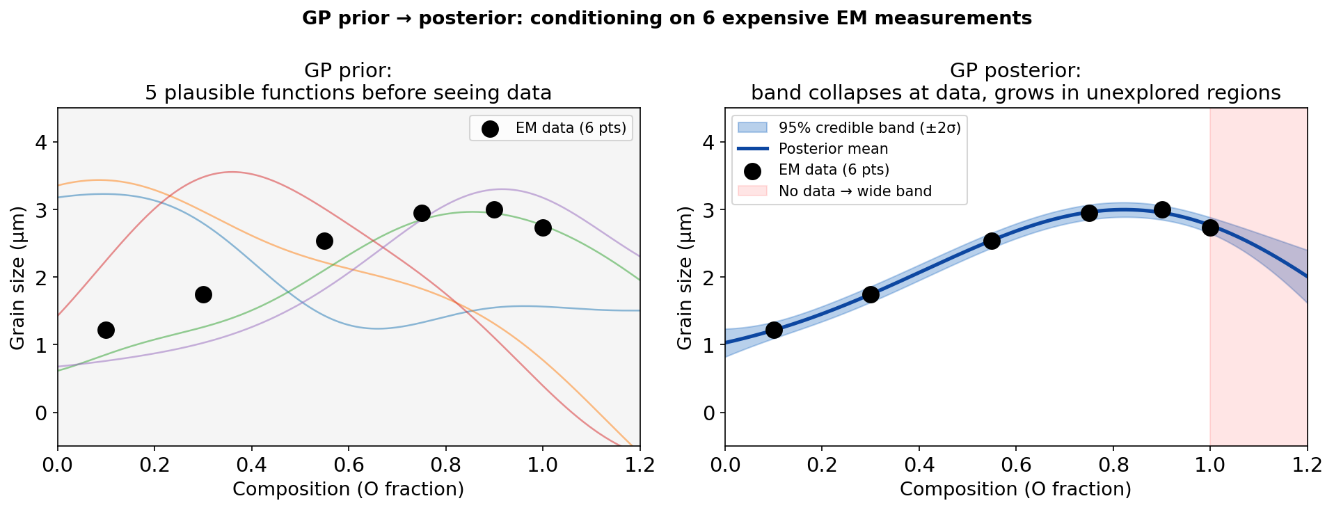
Left: GP prior — plausible curves before any EM data. Right: posterior after 6 EELS measurements (black) — curves pass near the observations; beyond x=1.0 (red shading) the band widens back toward the prior.

• Left panel first (prior): each coloured curve is one plausible “model” of Fe³⁺ fraction vs composition — all smooth (RBF), all on the same vertical scale (σ_f), all disagreeing because we have seen no data. The width of the cloud at any x is the prior variance σ_f².
• Right panel: the central picture of the GP block. Tight bundle at the data, fanning out to the right: “the GP knows what it doesn’t know — and says so.”
• Conditioning a joint Gaussian on some of its components gives another Gaussian: the posterior is again a GP, no approximation. This closure is why GPs are “exact Bayesian” regressors.
• Ask: “where would the GP tell you to measure next?” → the red region. That is the BO hook for later today.

The two GP posterior formulas

With noisy observations \(y_i = f(\mathbf{x}_i) + \epsilon_i\), \(\epsilon_i \sim \mathcal{N}(0,\sigma_n^2)\), kernel matrix \([\mathbf{K}]_{ij} = k(\mathbf{x}_i,\mathbf{x}_j)\) and \([\mathbf{k}_*]_i = k(\mathbf{x}_*,\mathbf{x}_i)\):

\[\boxed{\mu_*(\mathbf{x}_*) = \mathbf{k}_*^\top (\mathbf{K} + \sigma_n^2 \mathbf{I})^{-1} \mathbf{y}}\]

\[\boxed{\sigma_*^2(\mathbf{x}_*) = k(\mathbf{x}_*,\mathbf{x}_*) - \mathbf{k}_*^\top (\mathbf{K} + \sigma_n^2 \mathbf{I})^{-1} \mathbf{k}_*}\]

• Mean: a kernel-weighted vote of the training outputs. Variance: prior variance minus what the data explain — never increases with more data.
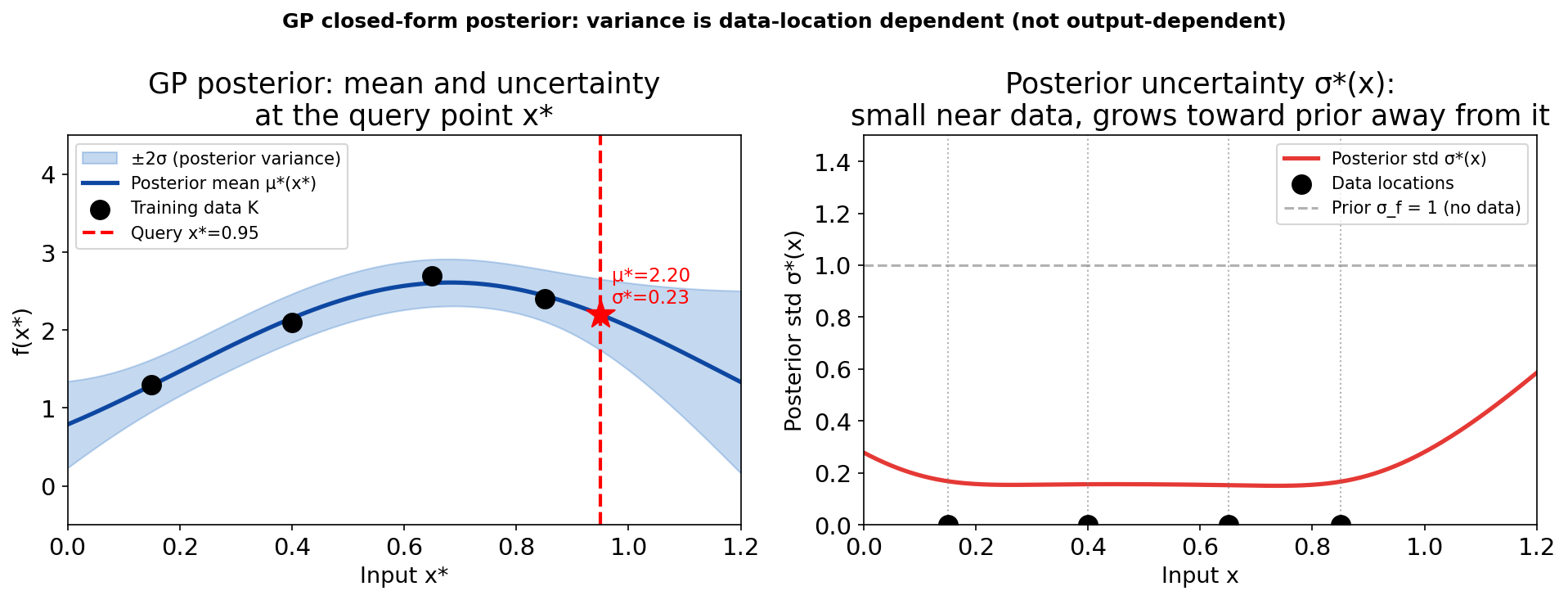
• \(\sigma_*^2\) depends only on where we measured, not on the \(y\) values → we can plan uncertainty reduction before measuring.
• Far from all data \(\mathbf{k}_* \to \mathbf{0}\) ⇒ \(\sigma_*^2 \to \sigma_f^2\): the GP reverts to the prior — uncertainty balloons. Cost: \(O(N^3)\) Rasmussen, Carl Edward et al., (2006).
• Aleatoric ↔︎ \(\sigma_n^2\) (WhiteKernel); epistemic ↔︎ the posterior variance of \(f\) — the decomposition from earlier, exactly.

• These two boxes are the highest-yield formulas of the lecture — students will be asked to reproduce and interpret them.
• Mean as a sentence: “close training points vote strongly, far ones barely vote; far from all data, the mean returns to the prior mean 0.”
• Variance as a sentence: “prior uncertainty minus the variance explained by the N observations.”
• The “depends only on x locations” property is the theoretical basis for active learning and experimental design.
• \(\sigma_n^2 \mathbf{I}\) is also the regulariser: without it the GP interpolates exactly through noisy points (and the matrix can be ill-conditioned — Week 3 conditioning callback).

The key intuition: uncertainty balloons away from data

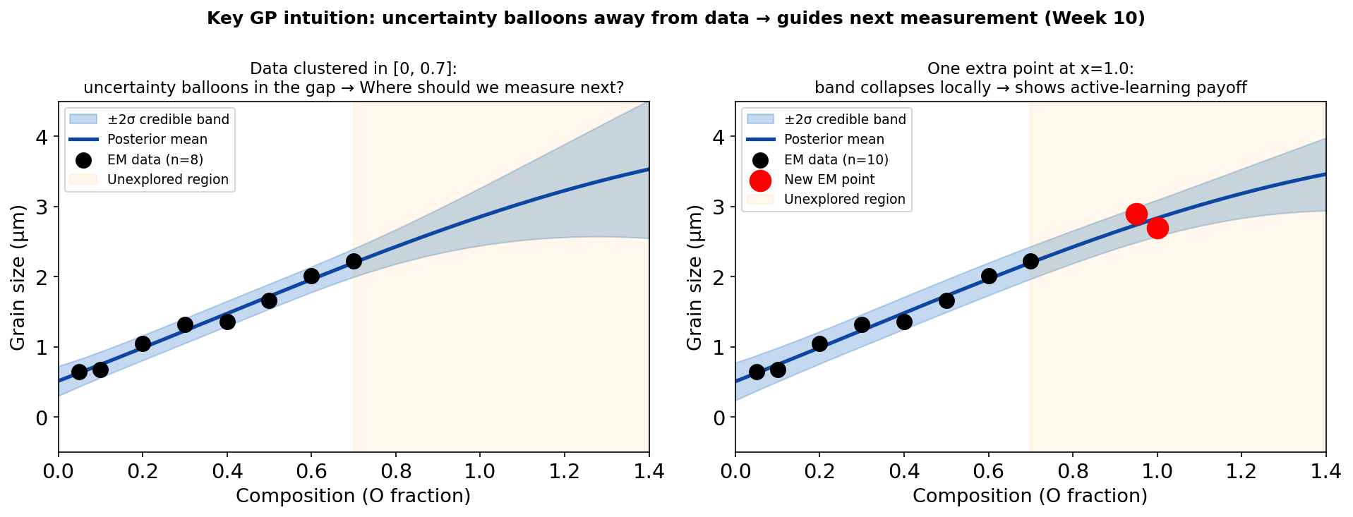
Illustration: left — GP fitted to 8 measurements clustered in [0, 0.7]; the 95% band widens rapidly beyond the data (red). Right — after one extra measurement at x=1.0 the band collapses locally while distant regions stay uncertain. In the notebook (EELS example, SEED=42) σ* at x=1.15 drops from 0.197 to 0.100 (−49%).

• Emotional payoff of the GP block. “The blue band is the honest error bar; in the red region the GP has never been told anything — and says so.”
• Notebook numbers (Part A): σ* near data (x=0.659) = 0.0145, far (x=1.15) = 0.1966 — 13.5×. Adding x=1.0 cuts σ* at x=1.15 by 49%; near-data σ* barely changes (+6.5%).
• Contrast with a neural net: it extrapolates its value confidently; a GP extrapolates its prior uncertainty.
• “Always measure where σ* is largest” is the simplest active-learning rule. BO refines it.

Kernel length-scale: smoothness and honesty

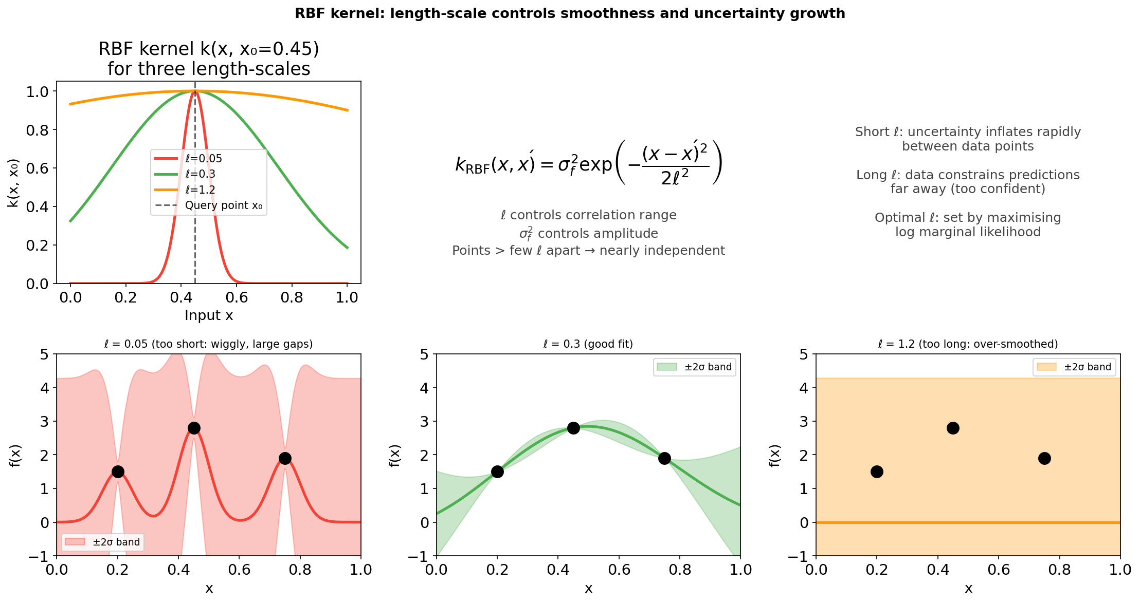
Top-left: RBF kernel for three length-scales. Bottom: GP posteriors with the same data and fixed ℓ. Short ℓ: wiggly mean, band inflates in every gap. Medium ℓ (≈ marginal-likelihood optimum): smooth mean, band opens only where data are missing. Long ℓ: over-smoothed and falsely confident extrapolation.

• Short ℓ is honest but useless; long ℓ is the dangerous one — narrow bands far from data.
• Notebook exercise A6 reproduces this with ℓ = 0.05, 0.3, 1.2.
• Transition: “How do we pick ℓ without looking at the answer?”

Hyperparameters, kernel families and practical tips

• Log marginal likelihood — maximise over \(\ell, \sigma_f, \sigma_n\): \[\log p(\mathbf{y}\mid\mathbf{X}) = -\tfrac12\mathbf{y}^\top(\mathbf{K}+\sigma_n^2\mathbf{I})^{-1}\mathbf{y} - \tfrac12\log|\mathbf{K}+\sigma_n^2\mathbf{I}| - \tfrac N2\log 2\pi\] data fit − complexity penalty: an automatic Occam’s razor Rasmussen, Carl Edward et al., (2006). In sklearn: GaussianProcessRegressor(n_restarts_optimizer=10).
• Kernel families: Matérn-5/2 (allows kinks — often better for materials), sums (trend + wiggle), products, ARD (one \(\ell_d\) per input dimension → irrelevant inputs get long \(\ell_d\)).
• Practice: normalise \(\mathbf{x}\) to [0,1] and \(y\) to zero mean / unit variance; check calibration on held-out data; multiple restarts (the likelihood is multimodal).

• The log-determinant term penalises flexible kernels (short ℓ) — complexity is paid for automatically, no separate regulariser.
• MFML callback: this is the “evidence” — the likelihood integrated over the function values.
• ARD is feature selection as a by-product: a huge optimised ℓ_d says “this input does not matter”.
• Multimodal likelihood: a short-ℓ “fit the noise” optimum and a long-ℓ “everything is noise” optimum can coexist; restarts guard against the wrong one.

GP scorecard: where GPs win and where they don’t

	Gaussian process	Deep neural network (+ ensemble)
Uncertainty	exact Bayesian (given the kernel)	add-on, approximate
Data regime	small, expensive (\(N \lesssim 10^3\))	large (\(10^4\)–\(10^7\))
Training cost	\(O(N^3)\) (sparse GPs: \(O(NM^2)\))	\(O(N)\) per epoch
Input dimension	struggles beyond ~10–20 raw dims	images, spectra natively
Features	hand-chosen via the kernel	learned
Interpretability	\(\ell, \sigma_f, \sigma_n\) physically meaningful	opaque weights

Experimental EM lives in the GP regime (5–500 expensive measurements) — unless inputs are images → deep kernel learning (later today).

• The GP is not universally better — it is better for the regime most common in experimental materials science: small N, low-dimensional inputs, need for calibrated intervals.
• Sparse / inducing-point GPs (GPyTorch, GPflow) push to N~10⁶ but are out of scope.
• The “image input” limitation is the cliffhanger for DKL: RBF on raw pixels is meaningless.
• Transition: “We have honest σ. Now: what do we do with it?”

From uncertainty to action: explore vs exploit

• Active learning — goal: an accurate model everywhere with few measurements. Acquisition: \(\alpha(\mathbf{x}) = \sigma_*(\mathbf{x})\) (pure exploration).
• Bayesian optimisation (BO) — goal: find the best setting (max SNR, max contrast) with few measurements. Acquisition must balance
  • exploitation — measure where \(\mu_*\) is high, and
  • exploration — measure where \(\sigma_*\) is high (maybe something better hides there).
• Same GP, different acquisition function. Next measurement: \(\mathbf{x}_{\text{next}} = \arg\max_{\mathbf{x}} \alpha(\mathbf{x})\) Shahriari, Bobak et al., (2016).
• BO-friendly objectives: expensive, no closed form, reasonably smooth, low-to-moderate dimension — i.e. almost every EM acquisition or process parameter.

• Week 8 callback: active labelling chose which images to label; here we choose which experiment to run. Same machinery.
• EM example: building a full Fe³⁺ map across compositions = active learning; finding the synthesis condition that maximises Fe³⁺ = BO.
• Ask the room: “why not always go to the highest-σ point?” — because we may waste budget mapping regions that are obviously bad.
• BO is pointless for functions you can evaluate in milliseconds — use gradients there.

The experiment-design problem in EM

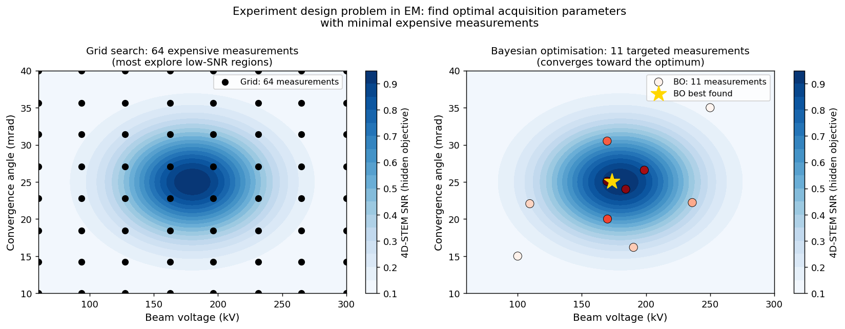
Left: a 64-point grid over (beam voltage × convergence angle) — most measurements land in low-SNR regions. Right: BO with 11 measurements (3 initial + 8 guided) converges toward the optimum (gold star, ≈180 kV, 25 mrad).

• A (S)TEM experiment has 50+ adjustable parameters; a 10-point grid per parameter is \(10^{50}\) measurements. Even a 2-D 10×10 grid at 1 h per point is 100 h of instrument time.
• BO propagates information from each measurement to its neighbours through the kernel, so the acquisition can jump straight to promising regions.
• In 2-D the kernel generalises with ARD — separate length-scales in voltage and angle, learned from data.

The Bayesian optimisation loop

1. Initialise: a few measurements at random / Latin-hypercube locations.
2. Fit the GP surrogate → \(\mu_*(\mathbf{x}), \sigma_*(\mathbf{x})\) everywhere (milliseconds).
3. Acquire: \(\mathbf{x}_{\text{next}} = \arg\max_{\mathbf{x}} \alpha(\mathbf{x})\), evaluated on a dense candidate grid (milliseconds).
4. Measure at \(\mathbf{x}_{\text{next}}\) — the expensive step (minutes to hours).
5. Update the dataset, go to 2 until the budget is spent. Report the best observed \(\mathbf{x}^+ = \arg\max_i y_i\).

• Outer loop = expensive experiments; inner loop = cheap GP algebra. All the cost lives in step 4.
• “The GP is a map, not the territory”: report the best observed measurement, not the maximum of the GP mean.
• Production libraries (BoTorch, scikit-optimize) use Cholesky updates (\(O(N^2)\) per new point) instead of refitting.

Acquisition functions: formalising explore vs exploit

• Upper Confidence Bound: \(\alpha_{\text{UCB}}(\mathbf{x}) = \mu_*(\mathbf{x}) + \kappa\,\sigma_*(\mathbf{x})\) — “optimism in the face of uncertainty”. \(\kappa=0\): pure exploitation; \(\kappa\to\infty\): pure exploration.
• Expected Improvement (current best \(f^+\), jitter \(\xi\)): \[\alpha_{\text{EI}}(\mathbf{x}) = (\mu_* - f^+ - \xi)\,\Phi(Z) + \sigma_*\,\phi(Z), \qquad Z = \frac{\mu_* - f^+ - \xi}{\sigma_*}\] how much improvement to expect; zero where the objective is already known (\(\sigma_*=0\)).
• Probability of Improvement: \(\alpha_{\text{PI}} = \Phi(Z)\) — how likely any improvement is; greedier than EI.
• All are closed-form in \((\mu_*, \sigma_*)\) → maximise by brute force on a grid in low dimension Shahriari, Bobak et al., (2016).

• UCB: “the mean here is 0.5 ± 0.3, so optimistically it could be 0.5 + 2×0.3 = 1.1.” Go to the most optimistic point.
• EI reads as: “improvement by at least ξ, weighted by how likely it is”. A high-σ point with a hopeless mean gets small EI.
• PI ignores magnitude and happily takes tiny improvements next to the current best.
• ξ in EI/PI plays the role of κ in UCB.

The BO loop in action on a multi-modal objective

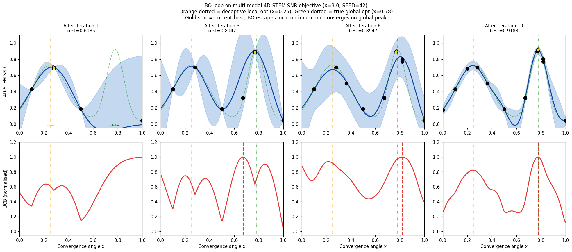
Four snapshots of BO (UCB, κ=3, SEED=42) on a synthetic 4D-STEM SNR vs convergence-angle curve with a broad deceptive local optimum (x≈0.25, orange) and a narrow global peak (x≈0.78, green). Blue: GP ±2σ; dashed red: next query. The loop escapes the local optimum and concentrates measurements on the global peak.

• Initial points sit near the deceptive local optimum (init best 0.6985). Iteration 1 goes to the uncertain boundary (x=1.0). Iteration 2 discovers the global peak (y=0.895). Later iterations refine near x=0.78.
• The true objective (shown for pedagogy) is never visible in a real experiment.
• Low κ (0.5) would have stayed near x=0.25 all 12 iterations.

BO vs random search: notebook numbers

• Budget: 3 initial + 12 iterations = 15 measurements (SEED=42).
• BO, UCB κ=3: best 0.9323 at x=0.776 (true optimum x=0.779, y=0.9205).
• Random: best 0.7229 at x=0.236 — stranded at the local optimum.
• κ matters: κ=0.5 → 0.744, κ=2 → 0.744 (stuck); κ=3 → 0.932, κ=5 → 0.933, EI (ξ=0.01) → 0.932.
• Lesson: on multi-modal objectives the amount of exploration matters more than the choice of acquisition function.

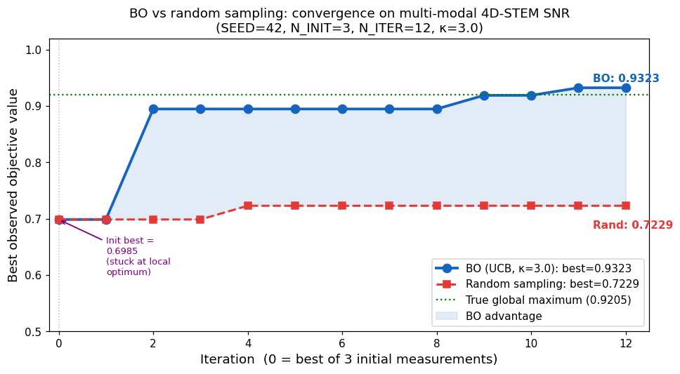
Best observed value vs iteration: BO (blue) jumps to the global-peak region at iteration 2 and refines to 0.9323; random search (red) stays near 0.72.

• These numbers are produced by notebook Part C and verified by assert checks there.
• +0.209 absolute (+29%) over random at equal budget; BO first gets within 0.05 of the true maximum at iteration 2 — genuine search, not luck at initialisation.
• Honest framing: κ=2 is the usual textbook default and it fails here within 12 iterations. Defaults are problem-dependent; the notebook exercise lets students see this.
• Transition: “This works for a 1-D knob. What if the input is an image patch?”

Deep kernel learning: GP uncertainty for image inputs

• Problem: predict a property at an unvisited probe position from its HAADF patch (1024-D). RBF on raw pixels measures noise, not structure.
• Deep kernel Wilson, Andrew G. et al., (2016): a neural feature map \(g(\mathbf{x};\mathbf{w})\), then a base kernel in the learned space: \[k_{\text{DKL}}(\mathbf{x},\mathbf{x}') = k_{\text{RBF}}\big(g(\mathbf{x};\mathbf{w}),\ g(\mathbf{x}';\mathbf{w})\big)\]
• Joint training: weights \(\mathbf{w}\) and GP hyperparameters maximise the same log marginal likelihood.
• Result: GP mean and σ on image inputs → acquisition functions work unchanged. Caveat: needs enough data to learn \(g\).

• Joint training = backprop through the GP formulas (Week 6 autograd). Needs tens–hundreds of points; tiny datasets overfit the feature map and σ becomes unreliable.
• MacKay’s old question (SS25 lecture): can we combine the representation learning of NNs with the calibrated uncertainty of GPs? DKL is one answer.
• The feature extractor decides which aspects of the patch matter for the target; the GP measures similarity in that space. They learn together.
• Architecture thread: the CNN from Week 7 becomes the kernel of a GP.
• Scalability: DKL with inducing points (KISS-GP) scales to large N; GPyTorch has it built in.

Automated 4D-STEM: the DKL active-learning workflow

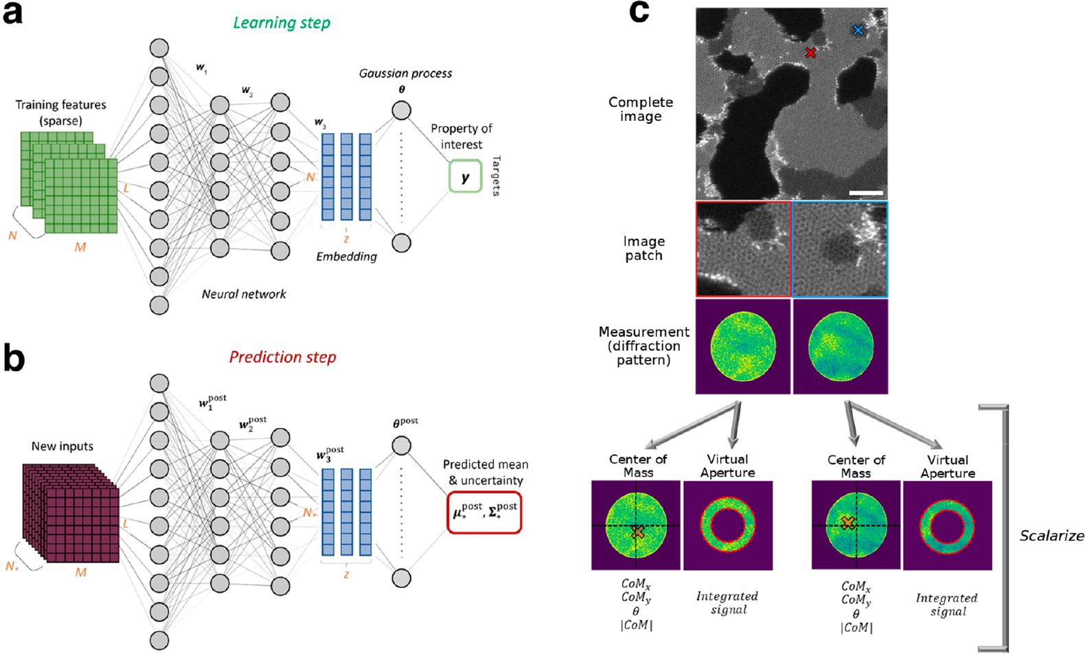
DKL workflow for automated 4D-STEM. (a) Learning: sparse HAADF patches → neural network embedding → GP → scalarised property y. (b) Prediction: mean and uncertainty for all unvisited patches. (c) Measurement: the diffraction pattern at the chosen position is scalarised (centre of mass, virtual aperture). Figure: Roccapriore et al., ACS Nano 16, 7605 (2022) Roccapriore, Kevin M. et al., (2022), doi:10.1021/acsnano.1c11118.

• Step 1: a fast, low-dose HAADF pre-scan of the whole field — the input for the feature extractor everywhere.
• Step 2: a few random 4D measurements to bootstrap the DKL model.
• Step 3: loop — refit DKL (~2 s on GPU), compute acquisition over all unvisited positions, move the probe, acquire one diffraction pattern, scalarise, repeat.
• The scalariser encodes the physics of interest: CoM magnitude (local electric field), CoM angle, Bragg-disc spacing (strain), integrated virtual-aperture signal. Changing the scientific question = changing one function.
• Between steps the beam is blanked — the specimen only sees dose where the algorithm decides it is worth it.

Automated 4D-STEM: results

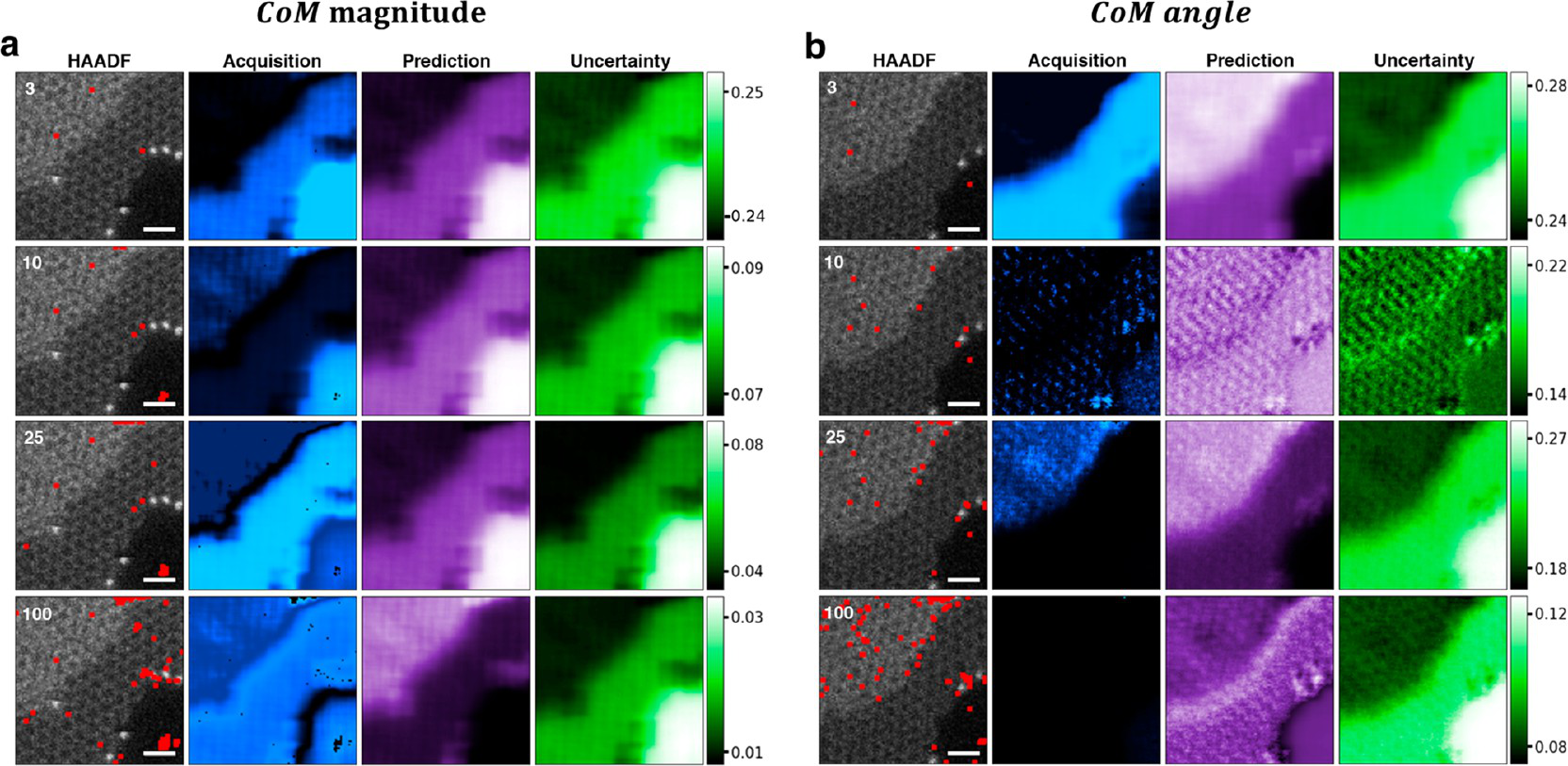
Experiment on graphene (Nion UltraSTEM 100): HAADF with visited points (red), acquisition, predicted CoM magnitude/angle and uncertainty after 3, 10, 25 and 100 steps. The acquisition concentrates on domain boundaries. Figure: Roccapriore et al., ACS Nano 16, 7605 (2022) Roccapriore, Kevin M. et al., (2022), doi:10.1021/acsnano.1c11118.

• Watch the uncertainty column shrink and the acquisition column concentrate at interfaces — the algorithm discovers that boundaries are where the physics changes.
• Headline: maps of comparable quality from a small fraction of probe positions → large dose savings. This matters most for beam-sensitive materials (MnPS₃ in the paper) where a full 4D scan would damage the specimen.
• Same approach used for autonomous discovery of bulk vs edge plasmons in EELS Roccapriore, Kevin M. et al., (2022), doi:10.1002/advs.202203422.
• Honest limits: the GP assumes smoothness in the learned feature space; sharp discontinuities the features miss are smoothed over, with deceptively low σ there. And the learned structure→property relation is itself a hypothesis that needs checking.

Choosing the right tool for acquisition

• Standard BO (GP + RBF/Matérn): 1–5 scalar knobs, 10–100 measurements.
• DKL active learning: image-patch or spectral inputs, \(10^2\)–\(10^4\) candidate positions.
• Sparse GPs: \(N > 10^3\), streaming data.
• Always log the trajectory: where the agent measured and where it did not — else invisible selection bias.
• Before trusting the loop: calibrated on this specimen? Still in-distribution? → next section.

• Examples of scalar knobs: voltage, convergence angle, dwell time, annealing temperature. DKL covers spatial field mapping.
• Most common student mistake in miniprojects: DKL on 5 data points. The feature map overfits and σ is meaningless.
• The selection-bias point is scientific integrity: if the agent skipped a region that contained the interesting defect, the published statistics are biased. Archive the full acquisition history.
• Transition: “An autonomous loop is only as trustworthy as its uncertainty. When does σ lie?”

When σ lies: out-of-distribution inputs

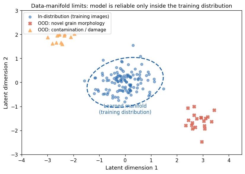
Training distribution (blue) vs OOD inputs: a novel grain morphology (red ×) and contamination/damage (orange). The model is only reliable inside the training region.

• Calibration ≠ OOD detection. Calibration: “given an in-distribution input, is my confidence honest?” OOD: “is this input like my training data at all?”
• Silent extrapolation: softmax stays at 0.95+ on a new detector; ensemble members all saw the same data and agree; a kernel that does not “see” the shift gives small σ.
• EM sources of shift: new microscope/detector, dose creep and beam damage, thicker specimen, contamination, a new alloy family.

• Two ideas students conflate. Both are mandatory; neither subsumes the other. A perfectly calibrated model still needs a detector that refuses to predict off-distribution.
• MG U14 example: a surrogate trained on oxides returns a confident posterior for a nitride — kernel-close, physically far. The small σ is meaningless.
• Dose creep: late frames of a long acquisition of a beam-sensitive specimen are OOD relative to early-frame training data.
• Softmax entropy is a poor OOD score: modern overconfident nets have low entropy on OOD inputs Hendrycks, Dan et al., (2017).

OOD scores and the trust gate

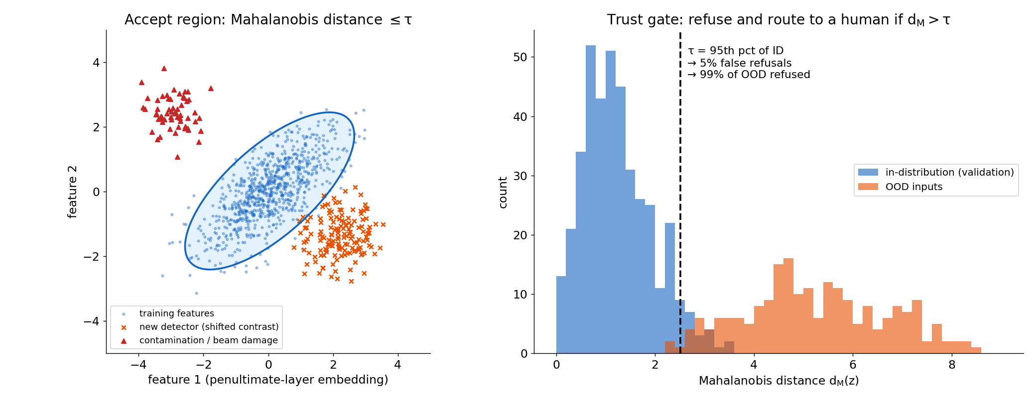
Left: training features (penultimate-layer embedding) with the Mahalanobis accept region; new-detector and contamination inputs fall outside. Right: Mahalanobis distances for in-distribution validation data vs OOD inputs; threshold τ at the 95th percentile of in-distribution → 5% false refusals, 99% of these OOD inputs refused (synthetic illustration, img/make_figures.py).

• Mahalanobis distance in feature space Lee, Kimin et al., (2018): fit mean and covariance of training embeddings; \(d_M(\mathbf{z}) = \sqrt{(\mathbf{z}-\boldsymbol\mu)^\top\boldsymbol\Sigma^{-1}(\mathbf{z}-\boldsymbol\mu)}\). Cheap, post-hoc, surprisingly effective on microscopy.
• Threshold selection: same operating-curve logic as reject-for-review. Choose τ at an acceptable in-distribution false-refusal rate (e.g. 95th percentile).
• Real OOD data will not separate this cleanly — the synthetic figure shows the procedure, not a performance promise. Validate on a genuinely different session or instrument.

The trust gate in practice

• Usable OOD scores: Mahalanobis distance of embeddings · ensemble disagreement · GP variance (in a kernel you trust) · autoencoder reconstruction error (Week 9) · nearest-neighbour distance in latent space.
• Gate rule: act automatically only if the uncertainty is small and the OOD score is low. Wide σ + low OOD → measure more (within known territory). Any + high OOD → refuse, route to a human or a cheap exploratory measurement.
• Use at least one score not derived from the model you are gating — surrogate-derived signals fail together.
• Audit trail per decision: model version, calibration set, OOD score and threshold, decision, human review. Periodic blind audits of confidently accepted cases.
• Trust is a system property, not a model property — combine calibration, conformal coverage and an OOD gate (MG U14).

• This slide is the Week 11 contribution to the course-wide explainability/trust thread (W4 coefficients, W5 SHAP, W7 saliency, W9 latent pitfalls, W10 attention, W11 uncertainty as a trust gate, W13 the E1–E6 ladder).
• Escalation pattern from MG U14: “wide σ + high OOD” = outside our coverage; “wide σ, low OOD” = uncertain within known territory → more data closes the gap. Different responses.
• Gate tightness depends on the cost of a wrong action: a destroyed beam-sensitive specimen → tight gate; a cheap re-scan → loose gate.
• Miniproject requirement callback: every miniproject must report uncertainty — this slide is the checklist.

Outlook: reinforcement learning and agents at the microscope

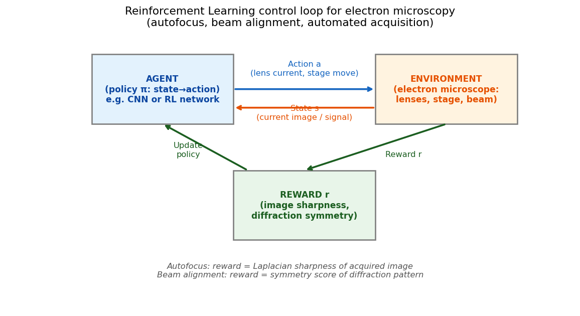
RL loop for an electron microscope: the agent observes a state (image, beam measurement), takes an action (lens current, stage move) and receives a reward (sharpness, diffraction symmetry, CoM magnitude).

• RL: learn a policy \(\pi(a\mid s)\) maximising \(\mathbb{E}\big[\sum_t \gamma^t r_t\big]\) from rewards — no labels Bishop, Christopher M., (2006).
• Time scales: BO for slow loops (one measurement per minutes–hours); RL policies for fast control (autofocus, stigmation, drift — every 0.1–10 s); DKL in between.
• Agents: LLM orchestrators calling BO, segmentation and analysis tools.
• Risks: reward hacking, sim-to-real gap, silent OOD, selection bias — every agent needs today’s trust gate.

• Agents: LLM-based orchestrators that plan sessions — an active research frontier (callback to the Week 10 LLM agents). Reward hacking example in one phrase: a “sharp” image of contamination.
• Keep this brief — an outlook, not examined in depth beyond the vocabulary (state, action, reward, policy) and the time-scale distinction.
• Control hierarchy: level 1 real-time corrections (autofocus RL, deployed in commercial software), level 2 session setup (alignment), level 3 experiment-level optimisation (BO, DKL). Level 1 failing silently corrupts level-3 measurements — monitor all levels.
• Reward hacking example: an autofocus agent maximising Laplacian variance can prefer sharp noise or contamination edges. Test policies on out-of-distribution images before deployment.
• The autonomous-lab vision (A-Lab, self-driving microscopes) is real but contested — MG U14 discusses the A-Lab debate; the lesson is the same: logs, audits, OOD gates.

Self-study notebook: GP → conformal → BO

• Notebook: notebooks/week11_gp_bo.ipynb — CPU, sklearn only, < 2 min
• Part A — GP regression: 8 simulated EELS measurements, posterior ±2σ, add a point, length-scale exercise.
• Part B — conformal: naive vs split conformal vs CQR on heteroscedastic data; exercise: α sweep and coverage under distribution shift.
• Part C — BO: UCB loop vs random at equal budget; exercise: vary κ, switch to EI.

Real-data extension (optional): MC-dropout U-Net on MetalDAM with reject threshold and tool-shift calibration — Ai4Mat companion notebook (ai4mat.datasets.MetalDAMDataset).

• Each part has a TODO exercise with a solution cell below; run the cells as-is first, then modify the “(try this yourself)” lines.
• Assert cells check non-trivial claims (e.g. BO beats random, CQR widens at high dose) on the fixed seed.
• The MetalDAM notebook needs a GPU for comfortable runtimes; it is optional.

Notebook key results (SEED=42)

• GP (Part A): optimised kernel \(0.476^2\,\mathrm{RBF}(\ell{=}0.373) + \mathrm{White}(1.7\times10^{-4})\); σ* near data 0.0145 vs far 0.1966 (13.5×); one extra point at x=1.0 → σ* at x=1.15: 0.197 → 0.100 (−49%).
• Conformal (Part B, α=0.1): naive training-residual band covers 0.78; split conformal 0.93; CQR 0.94 with a band 2.3× wider at high dose. Under dose shift (1.0–1.3) coverage falls to 0.70 — exchangeability broken.
• BO (Part C): UCB κ=3 best 0.9323 vs random 0.7229 at 15 measurements (+29%); κ ≤ 2 gets stuck at the local optimum (0.744).

• Every number on this slide is printed by the notebook’s final summary cell. If the notebook is re-run with a different sklearn version, re-check before teaching.
• The three numbers to remember: 13.5× (balloon), 0.78 vs 0.93 (don’t calibrate on training residuals), 0.93 vs 0.72 (BO vs random).

Summary

• Quantify: aleatoric (irreducible noise) vs epistemic (lack of knowledge). Ensembles and MC dropout give practical epistemic estimates for deep nets; per-pixel entropy + a reject threshold turns them into decisions.
• Certify: reliability diagram + ECE reveal over-confidence; temperature scaling fixes confidences post hoc; split conformal / CQR give distribution-free coverage if data are exchangeable.
• Model: GPs give exact, input-dependent uncertainty in closed form; σ* balloons away from data; the marginal likelihood picks the kernel.
• Act: BO = GP + acquisition (UCB/EI) in a closed loop; DKL extends it to image inputs → automated, dose-efficient 4D-STEM.
• Guard: OOD scores + σ form a trust gate; trust is a property of the system, logged and audited.

• Five verbs: quantify, certify, model, act, guard. Use them as the mental index for the exam.
• Link forward: the uncertainty ideas return in Weeks 12–13 as priors and posteriors in inverse problems, and in the E1–E6 explainability ladder synthesis.

Must-know takeaways

1. Aleatoric vs epistemic: “would more data of the same kind reduce it?”
2. Deep ensembles / MC dropout: spread of predictions = epistemic signal; model.eval() disables dropout.
3. Reliability diagram and ECE; temperature scaling changes confidence, not accuracy.
4. Split conformal: \(\hat q\) = \(\lceil (n{+}1)(1{-}\alpha)\rceil\)-th calibration score; guarantee needs exchangeability; CQR adapts the width.
5. GP posterior: \(\mu_* = \mathbf{k}_*^\top(\mathbf{K}+\sigma_n^2\mathbf{I})^{-1}\mathbf{y}\), \(\sigma_*^2 = k_{**} - \mathbf{k}_*^\top(\mathbf{K}+\sigma_n^2\mathbf{I})^{-1}\mathbf{k}_*\).
6. BO loop + UCB \(\mu_*+\kappa\sigma_*\); too little exploration → stuck in local optima.
7. DKL = NN feature map inside a GP kernel → BO on image patches (automated 4D-STEM).
8. Calibration ≠ OOD detection; act only if σ is small and the OOD score is low.

• The full list with numbers is in the must-know document for the exam. Items 4 and 5 are “reproduce from memory” items.

Next week: Inverse problems I

• Today: we learned to be honest about what we don’t know — and to measure where it matters.
• Week 12 — Inverse problems I: regularisation, tomography & sensor fusion. Measurements \(\mathbf{y} = \mathcal{A}(\mathbf{x}) + \boldsymbol\epsilon\) rarely are the quantity we want: a tilt series encodes a 3-D structure, a HAADF + EDS pair encodes composition.
• Recovering \(\mathbf{x}\) is ill-posed — many \(\mathbf{x}\) fit the data. Priors and regularisers (Tikhonov, TV) pick a plausible one; the Bayesian view of today (prior × likelihood → posterior) is exactly the language we need.
• Preparation: finish notebook Parts A–C; revisit Week 3 (SVD, conditioning) — the small singular values return as the source of ill-posedness.

• Close the arc: “Week 11 gave us posteriors over functions. Week 12 asks for posteriors over images and volumes — with a physical forward model in the middle.”
• Tomography teaser: the Radon transform, the Fourier-slice theorem and the missing wedge — why a tilt series can never fill all of Fourier space.
• Sensor fusion teaser: combining a high-SNR HAADF image with a noisy, low-resolution EDS map — two likelihoods, one reconstruction.

Continue

• ← Previous: Unit 10 — Attention, transformers & graph networks for EM
• → Next: Unit 12 — Inverse problems I: regularisation, tomography & sensor fusion
• All courses

Backup slides

Material moved out of the 90-minute lecture path; useful for questions and self-study.

GP posterior in pictures

Left: posterior mean and ±2σ band for 4 EELS measurements. Right: posterior standard deviation σ*(x) alone — near zero at the measurement locations, rising toward the prior σ_f in unexplored regions. This σ-map is what active learning and BO consume.

• Right panel: the “uncertainty map”. No y-values are needed to draw it — only the x locations.
• It approaches but does not reach σ_f exactly within the plotted range; far enough away it does.

Three acquisition functions on the same GP posterior

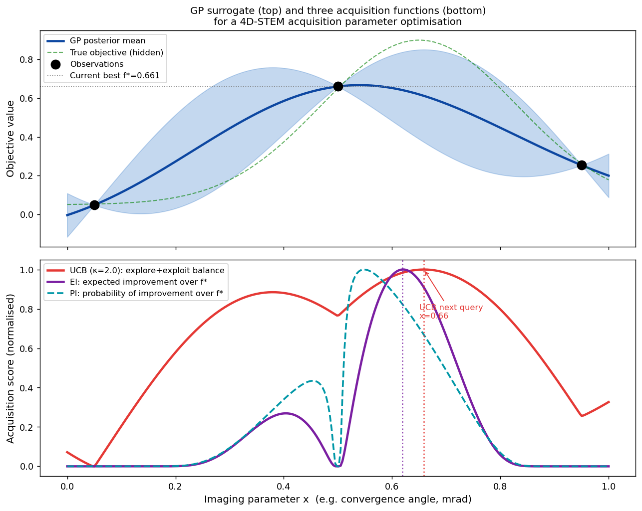
Top: GP surrogate after 3 measurements. Bottom: UCB (κ=2), EI and PI. All agree on the promising region but differ in how sharply they peak; each is maximised on a dense grid.

• The choice of acquisition function rarely changes the qualitative outcome on smooth problems; the amount of exploration does (BO vs random slide).
• Point at where each function peaks and why: UCB rewards σ more broadly, EI concentrates where improvement over f⁺ is plausible.

References

Pattern recognition and machine learning, Christopher M. Bishop.

Machine learning: A probabilistic perspective, Kevin P. Murphy.

Simple and scalable predictive uncertainty estimation using deep ensembles, Advances in neural information processing systems, Balaji Lakshminarayanan, Alexander Pritzel, & Charles Blundell.

Dropout as a Bayesian approximation: Representing model uncertainty in deep learning, Proceedings of the 33rd international conference on machine learning (ICML), Yarin Gal & Zoubin Ghahramani.

MetalDAM: Metallography dataset from additive manufacturing, ArcelorMittal & DaSCI Andalusian Research Institute.

A tutorial on the segmentation of metallographic images: Taxonomy, new MetalDAM dataset, deep learning-based ensemble model, experimental analysis and challenges, Information Fusion, Julián Luengo, Raúl Moreno, Iván Sevillano, David Charte, Adrián Peláez-Vegas, Marta Fernández-Moreno, Pablo Mesejo, & Francisco Herrera https://doi.org/10.1016/j.inffus.2021.09.018.

On calibration of modern neural networks, International conference on machine learning, Chuan Guo, Geoff Pleiss, Yu Sun, & Kilian Q. Weinberger.

A gentle introduction to conformal prediction and distribution-free uncertainty quantification, Foundations and Trends in Machine Learning, Anastasios N. Angelopoulos & Stephen Bates.

Conformalized quantile regression, Advances in neural information processing systems, Yaniv Romano, Evan Patterson, & Emmanuel J. Candès.

Gaussian processes for machine learning, Carl Edward Rasmussen & Christopher K. I. Williams.

Taking the human out of the loop: A review of Bayesian optimization, Proceedings of the IEEE, Bobak Shahriari, Kevin Swersky, Ziyu Wang, Ryan P. Adams, & Nando de Freitas.

Deep kernel learning, Proceedings of the 19th international conference on artificial intelligence and statistics (AISTATS), Andrew G. Wilson, Zhiting Hu, Ruslan Salakhutdinov, & Eric P. Xing.

Automated experiment in 4D-STEM: Exploring emergent physics and structural behaviors, ACS Nano, Kevin M. Roccapriore, Ondrej Dyck, Mark P. Oxley, Maxim Ziatdinov, & Sergei V. Kalinin https://doi.org/10.1021/acsnano.1c11118.

Physics discovery in nanoplasmonic systems via autonomous experiments in scanning transmission electron microscopy, Advanced Science, Kevin M. Roccapriore, Sergei V. Kalinin, & Maxim Ziatdinov https://doi.org/10.1002/advs.202203422.

A baseline for detecting misclassified and out-of-distribution examples in neural networks, International conference on learning representations (ICLR), Dan Hendrycks & Kevin Gimpel.

A simple unified framework for detecting out-of-distribution samples and adversarial attacks, Advances in neural information processing systems, Kimin Lee, Kibok Lee, Honglak Lee, & Jinwoo Shin.