Data Science for Electron Microscopy
Week 13: Inverse problems II: ptychography, generative priors & synthesis

Prof. Dr. Philipp Pelz

FAU Erlangen-Nürnberg

Institute of Micro- and Nanostructure Research

Recap: Week 12 and today’s question

• Week 12: every measurement follows \(\mathbf{y} = H\mathbf{x} + \boldsymbol{\epsilon}\); inversion is ill-posed (null space, small singular values), so we added priors (Tikhonov, TV, plug-and-play) and applied them to tomography and sensor fusion.
• The gap: (1) the forward models were linear — but a detector records \(|\psi|^2\) and loses the phase; (2) the priors were hand-designed.
• Today:
  1. Ptychography — a non-linear forward model made solvable by redundancy, with the right physics (strong phase, multislice) and the right solver (ePIE or autodiff).
  2. Generative priors — GAN → diffusion, diffusion posterior sampling, and physics constraints as the counterweight.
  3. Limits, causality and trust — when does a powerful prior invent structure?
  4. Course synthesis & exam preparation.

• Open by closing the Week 12 loop: “Last week every forward model was a matrix. Blur, projection, fusion — all linear. Today the forward model contains a modulus squared, and suddenly half the information (the phase) is gone at the detector.”
• Week 12 recap details (only if asked): L-curve / discrepancy principle for λ, Radon transform, Fourier-slice theorem, missing wedge, FBP vs iterative, HAADF + EDS fusion as one regularised objective.
• The Week 12 tomography material matters today: multislice ptychography has its own depth “missing wedge” (and ptychographic tomography combines both weeks — backup slide).
• This is the final lecture. Tell students up front that the last ~20 minutes are synthesis and exam preparation so they stay for it. Pacing: 2 minutes.

Learning outcomes

By the end of this lecture you can:

1. Write down the ptychographic forward model and explain why overlap makes phase retrieval over-determined.
2. State the strong-phase approximation, when it fails, and how multislice fixes it.
3. Formulate ptychography as loss minimisation and explain what autodiff buys over ePIE.
4. Explain GANs and diffusion models as learned priors and how diffusion posterior sampling works.
5. Distinguish soft (loss) and hard (architecture) physics constraints.
6. Diagnose hallucination and distribution shift before trusting a generative reconstruction.
7. Place the course’s methods on the E1–E6 explainability ladder.

• Outcomes 1–3 are the “physics + optimisation” half; 4–6 the “learned priors + trust” half; 7 is the course capstone.
• Exam hint: outcomes 2, 3, 4 and 6 map one-to-one onto must-know statements in _shared/exam_mustknow.md (Week 13 section).
• Pacing: 1 minute. Do not read them all aloud; point at 3, 4 and 7 as the new material.

Road map and self-study

• Road map (90 min): phase problem & ptychography (11) · object physics: strong phase & multislice (9) · ptychography as gradient descent (11) · learned priors: GAN → diffusion (10) · diffusion posterior sampling (5) · physics constraints (4) · risks, limits & causality (9) · course synthesis (7) · exam & miniproject (4) · wrap-up (8) · questions (8).
• Self-study: notebooks/week13_ptychography.ipynb — forward model + ePIE with an overlap sweep; the same model reconstructed by autodiff gradient descent; a low-dose exercise with a TV prior in one line of the loss.

• The two anchors for the whole lecture: (1) “ptychography flips the ill-conditioning — overlap makes the problem over-determined”; (2) “the more the prior carries, the more it can invent”. Everything else supports one of these.
• Notebook numbers (SEED=42, N_obj=48, N_probe=16): ePIE 40 iterations, step=4 (75 % overlap) 0.0991 → 0.0021; overlap sweep 4/6/8 px → 0.0021 / 0.0067 / 0.0091. Autodiff: full-batch Adam, lr 0.02, cosine schedule, 200 iterations, phase-only parameterisation \(O=e^{i\phi}\) — amplitude error 8.7e-5 vs 7.7e-4 (ePIE); aligned phase RMS 2.9e-4 vs 1.7e-3 rad. Low dose (100 e⁻/pattern): TV prior 0.103 → 0.080 rad.
• Timing plan (minute by minute, 90 min):
  • 0–4 admin: recap (2), outcomes (1), road map (1).
  • 4–13 phase problem & ptychography: phase problem (2.5), redundancy + overlap (2.5), forward model (2.5), ePIE (1.5) — then 13–15 ePIE convergence (2).
  • 15–24 object physics: weak → strong phase (2), SPA breaks → multislice (2.5), picture (2), depth missing wedge + thermal limit (2.5).
  • 24–35 gradient descent: loss (2), autodiff code (3), ePIE vs autodiff (2), what autodiff buys (1.5), low dose + TV (2.5).
  • 35–45 learned priors: hand-built → learned (2.5), GANs (2.5), GAN → diffusion (2), diffusion models (3).
  • 45–50 DPS: Bayes + algorithm (3), toy (2).
  • 50–54 physics constraints: PINN idea (2), soft vs hard (2).
  • 54–63 risks & limits: hallucination (2), distribution shift (2), when not to trust (2), limits (1.5), causality (1.5).
  • 63–70 synthesis: course arc (2), E1–E6 ladder (2), trust failures (1.5), five pillars (1.5).
  • 70–74 exam prep (2.5), miniproject (1.5).
  • 74–82 notebook pointer (1.5), summary (2), must-know (2), closing (1.5) + 1 buffer.
  • 82–90 slack for questions (~8 min; the estimator puts the lecture path at ≤ 85).
• Pacing: 1 minute. Transition: “Let us start with why phase is hard.”

The phase problem

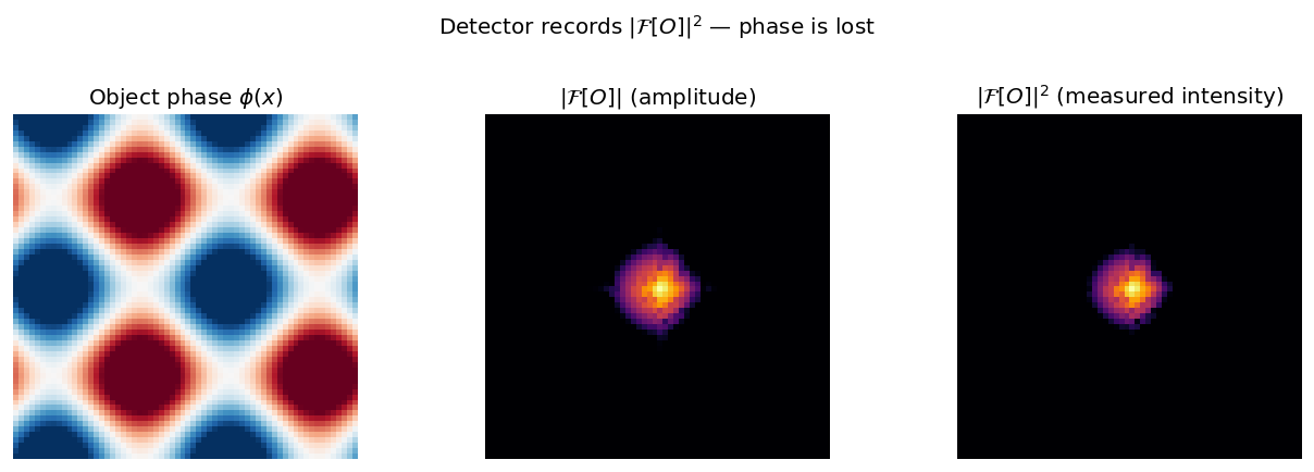
• Detectors record intensity \(|\psi|^2\); the phase \(\phi\) of \(\psi = |\psi|e^{i\phi}\) is discarded.
• In a thin specimen \(|\psi|\) is nearly uniform — almost all structural information sits in the phase.
• Recovering \(\phi\) from intensities is the phase problem.

Object phase (left), its Fourier amplitude (centre), and the recorded intensity \(|\mathcal{F}[O]|^2\) (right): the phase is gone.

• Key physical insight: TEM images are formed by interference of the electron wave. A pure phase object (zero absorption) produces zero amplitude contrast — an in-focus image of a thin specimen looks featureless even when real atomic structure exists. This is why defocus phase contrast, Zernike phase plates, DPC and ptychography all exist.
• Example: graphene (Z=6) shifts the electron phase by only ~0.1 rad per atom at 300 kV; HAADF contrast is tiny, phase contrast reveals each atom.
• Walk through the panels. Key phrase: “the detector is a phase eraser.” The map \(O \mapsto |\mathcal{F}[O]|^2\) is many-to-one (non-uniqueness) — Hadamard condition 2 violated in its most extreme form.
• Historical context: the phase problem in X-ray crystallography delayed protein structures for decades; Patterson and heavy-atom methods were the workaround.
• Transition: “How do we recover phase? We need more data — ptychography provides it.”

Redundancy is the key: overlapping probe positions

• One pattern: \(N^2\) intensities for \(2N^2\) real unknowns — under-determined.
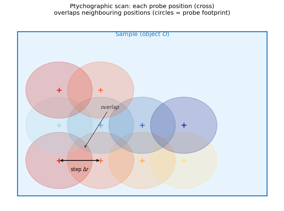
• Ptychography: scan the probe with a step smaller than the probe; neighbouring positions share most unknowns.
• 64×64 scan × 64×64 patterns ≈ 16.7 M measurements for a few \(10^4\) object pixels — massively over-determined. Rodenburg, John M. et al., (2007), doi:10.1103/PhysRevLett.98.034801
• Same redundancy idea as a tomographic tilt series (Week 12), applied to phase.

Probe centres (crosses) and footprints (circles): each object point is illuminated by several positions.

• Numbers: with a 64×64 scan at sub-probe step the object field is roughly (64·step + probe) pixels on a side — tens of thousands of unknowns vs 16.7 M measurements. The message is “orders of magnitude more data than unknowns”.
• GPS analogy: one satellite gives a sphere of possibilities, four give a point. Scan positions are the satellites of phase retrieval.
• Why overlap? If step = probe size, adjacent positions share no object pixels → each position is an independent under-determined problem. Overlap couples them. Standard ptychography uses 60–80 % overlap; the data set is a 4-D array (scan_y, scan_x, k_y, k_x) — “4D-STEM”.
• Cost vs benefit: more overlap = better reconstruction, but also more dose and data (dose–resolution trade-off: backup slide).

The ptychographic forward model

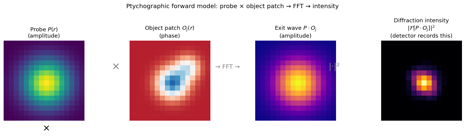
The four steps at scan position \(j\): (1) crop the object patch \(O_j(\mathbf{r})\); (2) multiply by the probe \(P(\mathbf{r})\) to form the exit wave; (3) FFT to the far field; (4) take \(|\cdot|^2\) to get the measured intensity. Steps 1–3 are reversible; step 4 is not — phase is lost.

\[I_j(\mathbf{k}) = \bigl|\mathcal{F}\bigl[P(\mathbf{r})\cdot O(\mathbf{r}-\mathbf{r}_j)\bigr]\bigr|^2\]

• Walk through each panel: probe amplitude, object patch phase, exit wave, diffraction intensity (log).
• The formula is the equation of today. Reconstruction = inverting this operator over all positions simultaneously.
• Note the product \(P\cdot O\): that is the thin-object (projection) assumption. We come back to it in a few slides — it is exactly the strong-phase approximation, and multislice replaces it.

Iterative phase retrieval: ePIE

• Alternate two constraints: Fourier amplitude must match \(\sqrt{I_j}\) (replace amplitude, keep phase); then propagate the correction back to the object.
• One ePIE step at position \(j\):
  1. Predict: \(\psi_j = P \cdot O_j\) → \(\Psi_j = \mathcal{F}[\psi_j]\)
  2. Replace amplitude: \(\Psi_j' = \sqrt{I_j} \cdot e^{i\arg \Psi_j}\)
  3. Back-propagate: \(\psi_j' = \mathcal{F}^{-1}[\Psi_j']\)
  4. Update object: \(O_j \leftarrow O_j + \beta \frac{P^*}{|P|^2_{\max}}(\psi_j' - \psi_j)\)
• Loop over positions in random order until the amplitude-consistency error stops falling. Maiden, Andrew M. et al., (2009), doi:10.1016/j.ultramic.2009.05.012

• Alternating projections: each constraint defines a set; if the sets intersect (enough overlap) alternating projections converge to the intersection.
• The update in step 4 is, up to the normalisation, a stochastic gradient step on \(\|\,|\Psi_j| - \sqrt{I_j}\,\|^2\) with respect to \(O_j\) — keep this in mind; it is the bridge to the gradient-descent section.
• Why shuffle positions? Same reason as SGD shuffles mini-batches (Week 4): avoids periodic artefacts and order bias.
• Blind ptychography adds the mirrored probe update \(P \leftarrow P + \beta\,(O_j^*/|O_j|^2_{\max})(\psi'_j-\psi_j)\).

ePIE convergence: error vs iteration

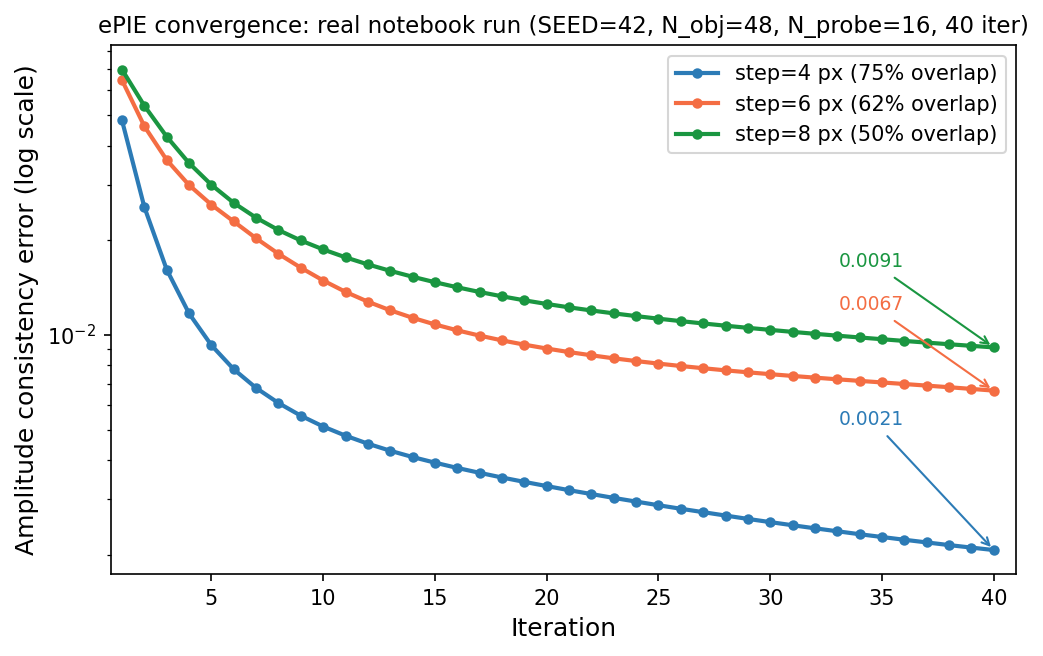
ePIE amplitude-consistency error vs iteration — output of week13_ptychography.ipynb (SEED=42, 40 iterations). Step 4 px (75 % overlap) → 0.0021; step 6 px (62 %) → 0.0067; step 8 px (50 %) → 0.0091. More overlap, lower error. Low error = self-consistent, not necessarily correct.

• The amplitude-consistency error is the normalised RMS difference between predicted and measured diffraction amplitudes — no ground truth needed. That is the metric you have in a real experiment.
• Numbers: 0.0991 → 0.0021 (step 4, ~48× below the flat-phase start), 0.1048 → 0.0067 (step 6), 0.1008 → 0.0091 (step 8). The ordering e4 < e6 < e8 is asserted in the notebook.
• Caveat to say aloud: low amplitude error = self-consistent, not necessarily correct. A wrong object that fits the data equally well is exactly the non-uniqueness problem — overlap is what removes it.
• Quality control in practice (backup slide): smooth plateauing error, residuals consistent with Poisson noise, stability across initialisations and half-sets.

The object model: from weak to strong phase

• Transmission function: \(O(\mathbf{r}) = e^{i\sigma V_p(\mathbf{r})}\), projected potential \(V_p = \int V\,dz\), interaction constant \(\sigma\).
• Weak-phase approximation (WPOA): \(\sigma V_p \ll 1 \Rightarrow O \approx 1 + i\sigma V_p\) — the forward model becomes linear (basis of CTF theory).
• Strong-phase approximation (SPA): keep the full exponential, \(\psi_{\text{exit}} = \psi_0\,e^{i\sigma V_p}\) — valid for phase shifts of several radians.
• SPA assumes the probe does not change shape inside the specimen (no propagation), pure phase object.
• In the notebook: parameterising \(O = e^{i\phi}\) is the SPA — a hard constraint \(|O|=1\).

• The order WPOA → SPA → multislice is a hierarchy of forward models of increasing fidelity and cost — the “choose the forward model that the physics demands” thread (Week 2 noise model, Week 12 linear operators).
• \(\sigma = 2\pi m e \lambda / h^2\) (relativistic \(m\)); at 300 kV roughly \(6.5\times10^{-4}\) rad V⁻¹ Å⁻¹. Not examined numerically. σ depends on beam energy.
• WPOA linearises; SPA keeps a single multiplicative phase screen — still a product \(P\cdot O\), so ePIE works unchanged. SPA also conserves \(|\psi|^2\) (no absorption).
• Exam hook: “Why does the weak-phase approximation linearise the forward model?” Answer: first-order Taylor expansion of the exponential.

When the strong-phase approximation breaks: multislice

• SPA fails for thick specimens (≳ 10–20 nm), low beam energies (< ~60 keV) and strong scatterers (heavy elements, channelling) — the probe changes shape inside the sample.
• Symptom: phase no longer scales linearly with thickness; ghost contrast at heavy columns.
• Multislice Cowley, J. M. et al., (1957), doi:10.1107/S0365110X57002194: cut the specimen into thin slices, transmit and propagate: \[\psi_{n+1} = p(\Delta z) \otimes \bigl[\psi_n \cdot e^{i\sigma V_n}\bigr], \qquad \mathcal{F}[p](\mathbf{k}, \Delta z) = e^{-i\pi\lambda\Delta z |\mathbf{k}|^2}\]
• Multislice ptychography reconstructs all slices \(V_1\ldots V_N\) Maiden, Andrew M. et al., (2012), doi:10.1364/JOSAA.29.001606 — a deep, differentiable chain of multiply → FFT → propagate → IFFT.

• The Fresnel propagator in Fourier space is a pure phase factor that grows with \(|\mathbf{k}|^2\) — high spatial frequencies are defocused more strongly per slice.
• The multislice forward model looks exactly like a neural network: repeated “multiply by learnable weights (the slice transmission), apply a fixed linear operator (propagation)”. That is why autodiff frameworks (next section) are the natural home for multislice ptychography.
• Historical note: Cowley & Moodie (1957) introduced multislice for dynamical electron scattering simulation; Maiden, Humphry & Rodenburg (2012) turned it into a reconstruction method.

Phase object vs multislice: a picture

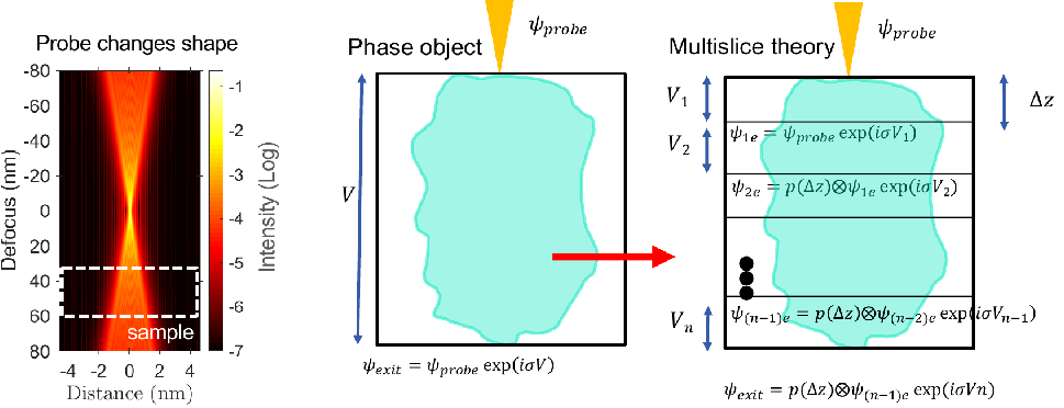
Left: the focused probe changes shape over tens of nm of defocus — comparable to the sample thickness (dashed box). Centre: the phase-object (SPA) model treats the whole specimen as one phase screen, \(\psi_{\text{exit}} = \psi_{\text{probe}}\,e^{i\sigma V}\). Right: multislice theory alternates transmission through thin slices \(V_n\) and Fresnel propagation \(p(\Delta z)\). Slide credit: D. Muller (M&M 2023), after Chen, Zhen et al. (2021), doi:10.1126/science.abg2533.

• Left panel is the physical argument: a convergent probe with ~20–30 mrad semi-angle has a depth of field of only a few nm. If the sample is 20 nm thick, the probe at the exit surface is not the probe at the entrance surface — the SPA assumption “probe does not change shape” is violated.
• Right panel = the formula on the previous slide, drawn.
• Chen et al. 2021 used multislice ptychography to reach lattice-vibration-limited resolution in ~20 nm thick PrScO₃ — next slide.

Depth sectioning, its missing wedge, and the thermal limit

• Depth information is carried only by high transverse frequencies (propagator phase \(\pi\lambda\Delta z|\mathbf{k}|^2\)).
• Low frequencies are nearly depth-invariant → a missing wedge in \(k_z\), as in limited-angle tomography (Week 12): depth resolution a few nm vs < 0.5 Å laterally.
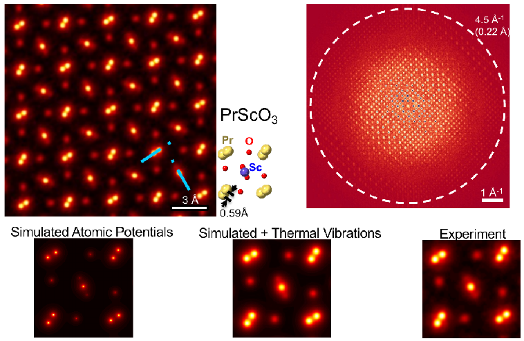
• Resolution limit: in PrScO₃ multislice ptychography reaches ~20 pm — set by thermal vibrations of the atoms, not the microscope. Chen, Zhen et al., (2021), doi:10.1126/science.abg2533

Multislice ptychography of PrScO₃: experiment matches simulation only once thermal vibrations are included. After Chen, Zhen et al. (2021), doi:10.1126/science.abg2533; slide credit D. Muller.

• Connect explicitly to Week 12: the missing wedge re-appears. Same mathematics — a region of Fourier space that the measurement never samples; a prior (regulariser) must fill it or it stays empty. \(\Delta z \propto 1/|\mathbf{k}_r|^2\).
• One can regularise along \(z\), e.g. with a Fourier-space weight \(W(\mathbf{k}) = 1 - \tfrac{2}{\pi}\arctan(\beta^2 k_z^2 / k_r^2)\), which damps structure along \(k_z\) not supported by lateral frequencies. Mention for recognition only.
• The thermal limit is a beautiful “limits” message: once the reconstruction is good enough, the specimen physics (atoms vibrate at room temperature, ~5–10 pm RMS) becomes the resolution limit. No algorithm can beat that without cooling the sample. Resolution history: electron ptychography now sits above aberration-corrected imaging and approaches this limit.
• Going 3-D (ptychographic tomography, our group’s work): backup slide.
• Transition: “How does such a reconstruction actually work? It is the same principle as training a neural network.”

Ptychography as loss minimisation

• Loss over all scan positions: \[\hat{\phi} = \arg\min_{\phi} \; \sum_j \Bigl\|\, \bigl|\mathcal{F}[P\cdot O_j(\phi)]\bigr| - \sqrt{I_j}\,\Bigr\|_2^2 \;+\; \lambda\,R(\phi)\]
• Data term from the noise model (Week 2): least squares on \(I\) (Gaussian), Poisson NLL (counts), or the amplitude loss on \(\sqrt{I}\) ≈ variance-stabilised Poisson — the common choice.
• Parameters: object, and optionally probe, scan positions, slice potentials, tilt angles.
• Solver: any gradient method (Week 4). ePIE ≈ SGD with batch size 1 and a hand-derived step \(\beta/|P|^2_{\max}\).

• This slide is the conceptual pivot: ptychography is ERM (Week 4) with a physics model instead of a neural network. \(\hat R(\phi)\) notation for the data term deliberately matches MFML.
• The amplitude loss: \(\sqrt{\text{Poisson}(\mu)}\) has variance ≈ 1/4 independent of μ for moderate counts (Anscombe) — the same variance-stabilising transform students met in Week 2. At very low dose the Poisson NLL \(\sum (\hat I - I\log\hat I)\) is statistically correct.
• Solvers: GD, SGD over positions (mini-batches), Adam, L-BFGS.
• The regulariser \(R\) is the Week 12 toolbox (Tikhonov, TV) — or a learned prior (later today).

Automatic differentiation: write the forward model, get the gradient

def forward(phi, probe, rows, cols):
    O = torch.exp(1j * phi)                    # SPA: pure phase object (hard constraint |O| = 1)
    exit_waves = probe * O[rows, cols]         # probe x all object patches at once
    return torch.abs(torch.fft.fft2(exit_waves))   # predicted diffraction amplitudes

phi = torch.zeros(N, N, requires_grad=True)
opt = torch.optim.Adam([phi], lr=0.02)
for it in range(200):
    loss = ((forward(phi, probe, rows, cols) - meas_amps) ** 2).sum()   # data fidelity
    loss = loss + lam_tv * tv(phi)                                      # prior: one extra line
    opt.zero_grad(); loss.backward(); opt.step()                        # autograd does the calculus

• loss.backward() differentiates through the FFT and the modulus — no hand-derived update. Kandel, Saugat et al., (2019), doi:10.1364/OE.27.018653
• Same pattern as training a network in Week 6 — the “network” is the physics.

• The notebook contains exactly this code.
• Two things to point at: (1) the parameterisation exp(1j*phi) is a hard physics constraint (we will name it again in the physics-constraints section); (2) the TV line — adding a prior to ePIE requires deriving a new algorithm, adding it here is one line.
• Complex gradients: PyTorch uses Wirtinger calculus internally; parameterising by the real \(\phi\) sidesteps the issue entirely.
• Kandel et al. 2019 is the reference paper that popularised AD as “a general framework for ptychographic reconstruction”.

ePIE vs autodiff gradient descent: same problem, two solvers

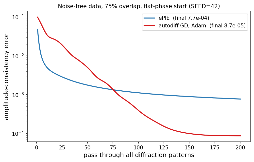
Amplitude-consistency error per pass through all 81 diffraction patterns (noise-free, 75 % overlap). Output of week13_ptychography.ipynb.

after 200 passes	ePIE	autodiff GD
amplitude error	\(7.7\times10^{-4}\)	\(8.7\times10^{-5}\)
aligned phase RMS	\(1.7\times10^{-3}\) rad	\(2.9\times10^{-4}\) rad
wall time (CPU)	4.5 s	9.3 s

• ePIE is fast early; full-batch Adam is more precise late (10× lower error).

• Numbers from the notebook run (SEED=42). ePIE makes 81 small updates per pass; Adam’s momentum + cosine schedule win late. Wall times depend on the machine; the ratio is what matters. After 40 passes ePIE is ahead (2.1e-3 vs 8.2e-3), but GD’s 40-iteration value comes from a schedule tuned for 200 iterations — not a fair early-stopping comparison, and say so.
• “Aligned phase RMS”: error inside the illuminated region after removing the global phase offset, which no intensity measurement can determine.
• The honest message: neither solver is magic; they minimise (almost) the same loss. The reason the field moved to autodiff is flexibility (next slide).

What automatic differentiation buys

• Flexibility: probe refinement, position correction, mixed probe states, multislice, tilt series — each is one more parameter or layer.
• Any loss, any optimiser: Poisson NLL at low dose; regularisers as loss terms; mini-batch SGD over millions of patterns on GPUs.
• Composability: a denoiser, a generative prior or a physics residual plugs into the same graph — the bridge to the rest of today.
• Costs: memory, hyperparameters, non-convexity — initialisation still matters.

• The composability point is why the rest of the lecture follows: once the reconstruction is a differentiable program, “prior” means “another differentiable term”, whether hand-designed (TV), physics (PINN residual) or learned (diffusion score).
• Non-convexity: the phase problem has trivial ambiguities (global phase, conjugate twin, translation) plus real local minima at low overlap. Good initialisation (e.g. a DPC or parallax estimate) is standard practice.
• Memory: for a 20-slice multislice model on 256×256 patterns with 10⁵ positions, storing intermediates dominates GPU memory; checkpointing trades compute for memory.
• Partial coherence as mixed states: \(I_j = \sum_k |\mathcal{F}[P_k \cdot O_j]|^2\) — trivial in an autodiff framework.

Low dose: a prior in one line of the loss

• Notebook exercise 2: Poisson noise, 100 e⁻ per pattern; aligned phase RMS error:

method	phase RMS [rad]
ePIE, 40 iterations	0.094
autodiff GD, \(\lambda_{TV}=0\) (200 it.)	0.103
autodiff GD, \(\lambda_{TV}=1\)	0.080
autodiff GD, \(\lambda_{TV}=8\)	0.140

• U-curve: too little prior fits noise; too much flattens the phase (bias) — the Week 12 \(\lambda\) trade-off.
• Early stopping is an implicit regulariser: ePIE at 40 iterations beats unregularised GD.
• The weaker the data, the more the prior has to carry.

• All numbers from the executed notebook (noise seed 0). At 10× the dose (1000 e⁻/pattern) the optimal \(\lambda_{TV}\) drops to ≈ 0.3: ePIE 0.037 rad, GD+TV(0.3) 0.032 rad.
• The sentence “the weaker the data, the more the prior has to carry” is the thread into the generative section: a diffusion prior at very low dose carries almost everything — that is where hallucination lives.
• Ask the room: “Why does TV hurt at large λ for this object?” Because the true phase is smooth Gaussian blobs, not piecewise constant — the prior is mis-specified. Priors encode assumptions; wrong assumptions bias the answer.
• Transition: “So far the prior was either nothing (overlap alone) or TV. What if we learn the prior from data?”

From hand-built regularisers to learned priors

• Regularisation = MAP: \[\min_{\mathbf{x}} \|H(\mathbf{x}) - \mathbf{y}\|^2 + \lambda R(\mathbf{x}) \;\Leftrightarrow\; p(\mathbf{x}) \propto e^{-\lambda R(\mathbf{x})}\]
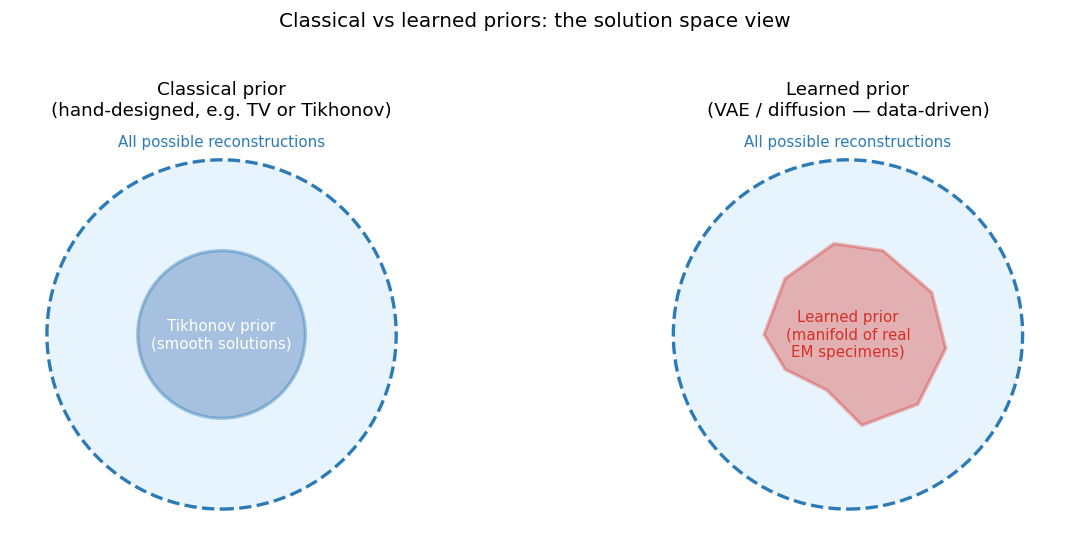
• Tikhonov, TV, positivity: hand-designed; none knows what real specimens look like.
• Two ways to do better: put known physics into the loss/architecture, or learn \(p(\mathbf{x})\) from data with a generative model.
• Week 12’s plug-and-play denoiser is the bridge: a diffusion model is a denoiser at every noise level.

Hand-designed prior: a simple set (left). Learned prior: an irregular manifold shaped by the training data (right) — accurate in distribution, dangerous outside it.

• The MAP ⇔ regularisation equivalence is the single most important bridge of the lecture. Write it on the board. Posterior ∝ likelihood × prior: the likelihood comes from the forward and noise models; the prior is the only place where “what specimens look like” enters.
• Prior spectrum from least to most data-dependent: hard constraints (positivity, \(|O|=1\)) → hand-crafted regularisers (TV) → physics residuals (PINN) → learned denoisers (PnP) → full generative models (diffusion).
• PnP recap (details on a backup slide): replace the proximal step of ADMM with any strong denoiser \(D_\sigma\) (BM3D, DnCNN, U-Net) Kamilov, Ulugbek S. et al., (2023), doi:10.1109/MSP.2022.3199595.
• Figure: if the test specimen is off the learned manifold, the prior forces the reconstruction onto it anyway — inventing structure that looks like training data. This is the hallucination mechanism; keep it in mind for the risk section.
• Generative families: VAE (Week 9: one-step, smooth latent, blurry), GAN, diffusion. VAE (2013) and GAN (2014) → diffusion (2020) became the default by 2022. MFML Unit 11 and MG Unit 12 have the derivations.
• Rule of thumb: little data + well-known physics → hand-designed/physics. Lots of in-distribution data + complex structure → learned prior.

GANs: an adversarial prior for sharp images

• Minimax game Goodfellow, Ian et al., (2014): \[\min_G \max_D \; \mathbb{E}_{\mathbf{x}\sim p_{\text{data}}}[\log D(\mathbf{x})] + \mathbb{E}_{\mathbf{z}}[\log(1 - D(G(\mathbf{z})))]\] generator \(G(\mathbf{z})\) maps noise to an image; discriminator \(D(\mathbf{x})\) says “real or fake”.
• Strength: sharp samples in one forward pass (no MSE blur); conditional GANs map low-dose → high-dose.
• As a prior: \(\hat{\mathbf{z}} = \arg\min_{\mathbf{z}} \|H(G(\mathbf{z})) - \mathbf{y}\|^2\) — the solution lies on the generator’s manifold.
• Failure modes: unstable training, mode collapse, and no likelihood.

• Do not derive the optimal discriminator; state the result: at the optimum \(D \equiv 1/2\) and \(G\) reproduces the data distribution.
• Unstable training: two players, no single loss to monitor. No likelihood: you cannot ask “how probable is this reconstruction?”
• Mode collapse in EM terms: a GAN trained on perfect SrTiO₃ reconstructs any noisy perovskite as a perfect lattice — defects are “off-mode” and get erased.
• Latent-space search (Bora et al.’s “compressed sensing with generative models”) — powerful, but if the true object is not in the generator range the error cannot go to zero.
• Transition: “These failure modes are why the field moved to diffusion.”

From GANs to diffusion: why the field moved

• Stable training: a plain regression loss (predict the noise) — one network, no adversary.
• Mode coverage: likelihood-based objective → diverse samples, no mode collapse.
• A score, not just a sampler: diffusion gives \(\nabla_{\mathbf{x}} \log p_t(\mathbf{x})\) at every noise level — what Bayesian inverse problems need. Song, Yang et al., (2021)
• Price: slow sampling — tens to hundreds of network evaluations vs one for a GAN.

• This is the pedagogical “GAN → diffusion” arc required by the curriculum. Emphasise the score bullet: a GAN gives samples, a diffusion model gives the gradient of the log prior.
• Loss curves you can read (Week 6 diagnostics apply).
• Faster samplers: DDIM, latent diffusion, flow matching, consistency models. Flow matching learns a velocity field instead of a noise predictor (MFML U11). Mention only.
• In materials science diffusion generates crystal structures (MatterGen, DiffCSP, MG Unit 12) and microstructures; in EM it drives denoising and super-resolution (applications: backup slide).

Diffusion models: forward noising, learned reverse

• Forward process (fixed): add Gaussian noise with schedule \(\beta_t\); closed-form marginal Ho, Jonathan et al., (2020) \[q(\mathbf{x}_t \mid \mathbf{x}_0) = \mathcal{N}\bigl(\sqrt{\bar\alpha_t}\,\mathbf{x}_0,\,(1-\bar\alpha_t)\mathbf{I}\bigr), \qquad \bar\alpha_t = \textstyle\prod_{s\le t}(1-\beta_s)\]
• Training: form \(\mathbf{x}_t = \sqrt{\bar\alpha_t}\mathbf{x}_0 + \sqrt{1-\bar\alpha_t}\,\boldsymbol\epsilon\) and minimise \[\mathcal{L} = \mathbb{E}\,\bigl\|\boldsymbol\epsilon - \boldsymbol\epsilon_\theta(\mathbf{x}_t, t)\bigr\|^2\] with a U-Net (Week 7) that predicts the noise.
• Sampling: start from \(\mathbf{x}_T\sim\mathcal{N}(0,I)\), denoise step by step — coarse structure first.
• Score: \(\nabla_{\mathbf{x}_t}\log p_t(\mathbf{x}_t) \approx -\boldsymbol\epsilon_\theta(\mathbf{x}_t,t)/\sqrt{1-\bar\alpha_t}\).

• Closed-form marginal means you never simulate the forward chain during training — pick any \(t\) directly. Sample \(\mathbf{x}_0\), \(t\), \(\boldsymbol\epsilon\sim\mathcal{N}(0,I)\).
• The noise-prediction network is literally a denoiser at noise level \(\sqrt{1-\bar\alpha_t}\) — the PnP link.
• Score connection: for Gaussian corruption, predicting the noise is equivalent to predicting the score (denoising score matching). Not derived here; MFML U11.
• Transition: “Now combine the prior score with the measurement.”

Diffusion posterior sampling (DPS)

• Bayes for scores — the normaliser drops out: \[\nabla_{\mathbf{x}_t}\log p_t(\mathbf{x}_t\mid\mathbf{y}) = \underbrace{\nabla_{\mathbf{x}_t}\log p_t(\mathbf{x}_t)}_{\text{learned prior score}} + \underbrace{\nabla_{\mathbf{x}_t}\log p_t(\mathbf{y}\mid\mathbf{x}_t)}_{\text{data consistency (intractable)}}\]
• DPS Chung, Hyungjin et al., (2023): evaluate the likelihood at the clean-image (Tweedie) estimate \(\hat{\mathbf{x}}_0 = (\mathbf{x}_t - \sqrt{1-\bar\alpha_t}\,\boldsymbol\epsilon_\theta)/\sqrt{\bar\alpha_t}\).
• Each reverse step: usual denoising step → \(\mathbf{x}'_{t-1}\), then \[\mathbf{x}_{t-1} = \mathbf{x}'_{t-1} - \zeta_t\,\nabla_{\mathbf{x}_t}\bigl\|\mathbf{y} - H(\hat{\mathbf{x}}_0)\bigr\|\]
• Works for non-linear \(H\) (ptychography): autodiff through network and physics. Repeat with new seeds → an ensemble of posterior samples.

• The Bayes-for-scores line is exam-level: “posterior score = prior score + likelihood score”. Everything else is the approximation that makes it computable. Goal: sample \(p(\mathbf{x}\mid\mathbf{y})\), not one MAP estimate.
• Tweedie (details on a backup slide): \(\hat{\mathbf{x}}_0 = \mathbb{E}[\mathbf{x}_0\mid\mathbf{x}_t]\), the network’s best guess of the clean image — blurry early, sharp late. It lets us push a clean estimate through the physical \(H\) at every step even though \(\mathbf{x}_t\) is noisy.
• Algorithm in words: start from noise; for t = T…1: prior step with \(\boldsymbol\epsilon_\theta\), clean estimate, data step; return \(\mathbf{x}_0\).
• Compare with PnP: data step + denoiser step, but with a noise schedule and injected randomness → samples instead of one point estimate.
• \(\zeta\) is a step size; DPS normalises it by the residual norm. It is not a calibrated posterior sampler — see the toy on the next slide.
• Cost: one network forward + backward per step, 100–1000 steps per sample, several samples → minutes to hours.
• The ensemble spread is a (heuristic) uncertainty map — a direct link to Week 11 ensembles. Variants to name only: ΠGDM, DDRM, latent DPS.
• DPS was introduced by Chung et al. (ICLR 2023) and demonstrated on phase retrieval and non-uniform deblurring.

DPS on a toy: what the data fix and what the prior decides

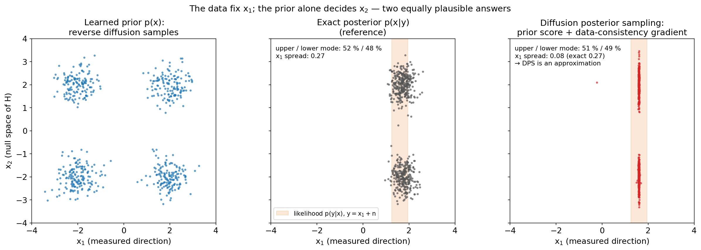
2-D toy with an exact prior (four Gaussian “structural variants”) and exact noised scores. We observe only \(x_1\) (a projection, \(H=[1\;0]\)); \(x_2\) lies in the null space of \(H\). Left: unconditional reverse diffusion reproduces the prior. Centre: exact posterior. Right: DPS samples. Generated by img/make_figures.py.

• Read the figure as a lesson about null spaces: the measurement pins \(x_1 \approx 1.6\); nothing in the data says anything about \(x_2\). The posterior has two modes (upper and lower) of equal weight — both answers are equally consistent with the data. The prior alone decides.
• DPS gets the important thing right (both modes, ≈ 50/50) but its spread along the measured direction is too narrow (0.08 vs 0.27 exact) and slightly shifted to the measured value: DPS is an approximation, not an exact posterior sampler.
• EM translation: \(x_2\) could be “is there an atom at the centre of this cell?” at a dose where the data cannot tell. A single sample would confidently show one answer. Only the ensemble reveals that there are two.
• This is the hallucination slide in disguise — the risk section returns to it.
• Transition: “Before the risks: the other kind of prior — physics.”

Physics-informed learning: the key idea

• Generative priors know data, not physics. Physics-informed learning adds a known equation, conservation law or symmetry to the objective. Raissi, Maziar et al., (2019), doi:10.1016/j.jcp.2018.10.045
• PINN loss: \[\mathcal{L}(\theta) = \underbrace{\tfrac{1}{N}\textstyle\sum_i \|f_\theta(\mathbf{x}_i) - y_i\|^2}_{\text{data fidelity}} + \lambda\,\underbrace{\tfrac{1}{M}\textstyle\sum_m \|\mathcal{N}[f_\theta](\mathbf{x}_m)\|^2}_{\text{physics residual}}\]
• Small-data advantage: the residual constrains the solution where there are no data.

• From MFML U13 and the ML-PC PINN unit. \(\mathcal{N}\) is the differential operator; derivatives by autodiff w.r.t. the inputs. Collocation points \(\mathbf{x}_m\) need no labels.
• EM reading: data term = “reproduce the measurements”; physics term = “obey the known law” (e.g. Poisson’s equation for the potential, a diffusion equation for in-situ kinetics).
• The λ knob: λ=0 → pure data fitting; λ→∞ → pure physics. Always monitor both terms: small residual + large data error → over-trusting physics; small data error + large residual → fitting noise.
• Optimisation pathologies: very different term scales, stiff PDEs, spectral bias of MLPs. Loss weighting and curricula help.
• Ptychography itself is “physics-informed” in the strongest sense: the entire model is the physics, only the object is learned.
• Complementarity: physics knows the law but not the typical specimen; generative priors know typical specimens but not the law. DPS with a physical \(H\) combines both — the current frontier.

Soft vs hard physics constraints

• Soft (penalty): add \(\lambda\|\text{violation}\|^2\) to the loss — flexible, only approximately satisfied, λ must be tuned.
• Hard (parameterisation / architecture): make violations impossible.
  • \(O = e^{i\phi}\) guarantees \(|O|=1\) (notebook); positivity via softplus.
  • Boundary conditions — Lagaris substitution Lagaris, Isaac G. et al., (1998): \(\hat u(x) = A(x) + B(x)\,N_\theta(x)\).
  • Symmetry: equivariant architectures (CNN, GNN; Weeks 7, 10).
• Hard constraints are exact but only as good as their physics: wrong physics (SPA for a thick sample) biases the result confidently.

• The hard/soft distinction is exam-relevant and ties the course together: architecture as inductive bias (W6→W7→W10) is the hard-constraint side of the same coin.
• Lagaris: \(A\) satisfies the BC and \(B=0\) on the boundary. Example from MFML U13: for \(x'=x\), \(x(0)=1\), use \(\hat x(t) = 1 + t\,N_\theta(t)\) — the initial condition holds for any weights. Normalisation: softmax.
• Rule: if a constraint is certainly true, hard-code it; if it is approximate (SPA for a 30 nm crystal), keep it soft — or better, upgrade the forward model (multislice).
• Wrong physics examples: wrong symmetry, SPA for a thick sample, ignoring inelastic scattering — the reconstruction still fits the data. Hard-coding \(|O|=1\) for an absorbing specimen biases the phase.
• Transition: “Now the honest part — how do powerful priors fail in practice?”

The honest risks: hallucination in EM

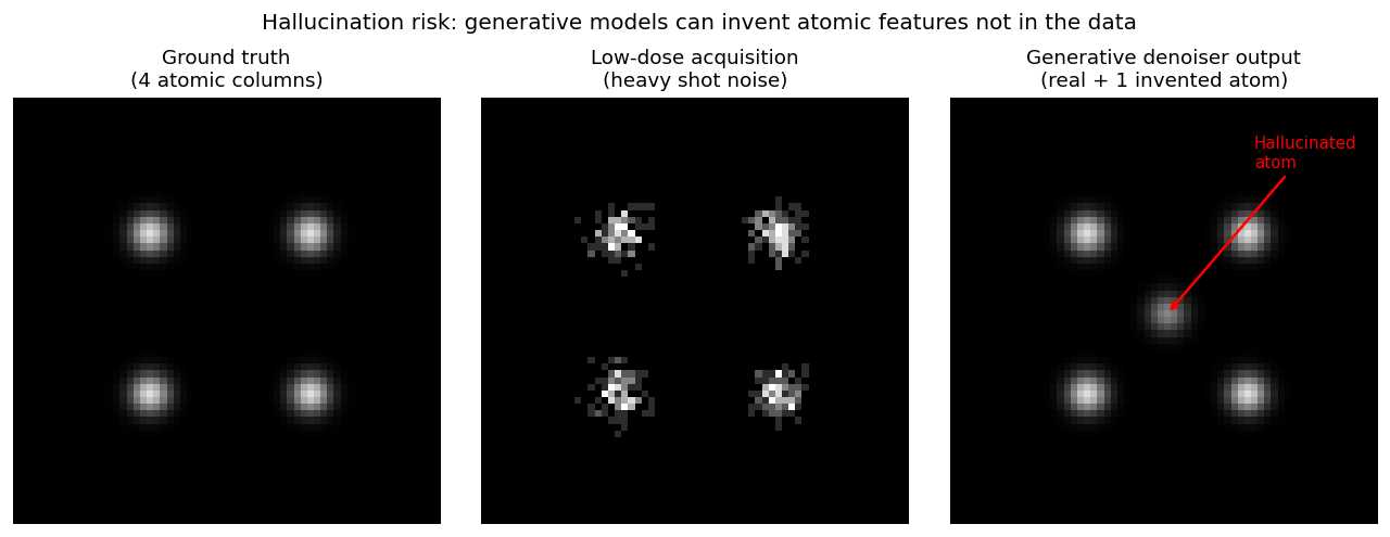
Low-dose HAADF image (centre) of four real atomic columns. A generative denoiser (right) recovers them but also invents a fifth (red arrow) — no basis in the ground truth (left). The prior places an atom where one “usually is”.

• Walk through the three panels. The noisy centre region gave slight support for “something”; the prior filled in the most probable completion — which was wrong.
• Connect to the DPS toy: the centre of the cell is a null-space direction at this dose. The posterior is bimodal (atom / no atom); a single sample shows one mode with full confidence.
• Every application (denoising, super-resolution, missing-wedge inpainting, synthetic training data) raises the same question: did the network reveal structure or invent it? Low dose = weak likelihood = strong prior = high risk.
• Prevention: (1) ensembles of posterior samples; (2) residual checks; (3) physics constraints; (4) high-dose validation of the key feature.

Distribution shift: when training data do not match the specimen

• Prior learned from \(p_{\text{train}}\), specimen from \(p_{\text{test}} \neq p_{\text{train}}\) — the most common cause of hallucination.
• EM examples: prior trained on perfect SrTiO₃ smooths away a grain boundary; Au-trained prior gives Pt columns Au-like contrast; simulation-trained prior on experimental data.
• Detect: residual \(\mathbf{y} - H(\hat{\mathbf{x}})\) should look like noise; OOD scores (Week 11); disagreement with a prior-free (ePIE / TV) reconstruction.
• Mitigate: diverse training data, physical forward model in the loop (DPS, not image-to-image), independent validation.

• Distribution shift is the most common real-world failure — different microscope, preparation, dose, orientation.
• Simulation → experiment: you partly measure how well the simulation matches reality (inverse crime in reverse).
• The “compare with a prior-free reconstruction” check is cheap and powerful: features present in the generative result but absent in a TV reconstruction of the same data deserve suspicion.
• Link to Week 11: the OOD gate and conformal coverage both assume exchangeability with the calibration data — the same assumption the generative prior silently makes.

When NOT to trust a generative reconstruction

• Red flags:
  1. Very low dose and a suspiciously clean, noise-free result.
  2. A feature of a type absent from the training data.
  3. Structured residuals.
  4. The feature would be the headline result of your paper.
• Checks:
  1. Ensemble agreement across posterior samples / seeds.
  2. Normalised residuals \(r_i = (y_i - H(\hat{\mathbf{x}})_i)/\sqrt{H(\hat{\mathbf{x}})_i} \sim \mathcal{N}(0,1)\).
  3. Agreement with a prior-free (ePIE / TV) reconstruction.
  4. Key features confirmed at higher dose or independently.

• The “headline result” red flag is intentionally provocative: priors have most influence exactly where the data are weakest, and that is often where the surprising finding sits. Low dose ≈ < 10² e⁻/Ų.
• The normalised residual check (Poisson): mean ≠ 0 → systematic bias; variance < 1 → over-fitting; variance > 1 → under-fitting or wrong noise model.
• Uncertainty quantification: a single reconstruction has no error bar. Posterior ensembles (heuristic — DPS under-disperses, as the toy showed); classical alternatives: half-set reconstructions (odd/even positions), bootstrap over patterns, Laplace approximation around the MAP (Week 11). Physics constraints shrink the space of possible hallucinations Pelz, Philipp M. et al., (2023), doi:10.1038/s41467-023-43634-z.
• Report: method, training data, dose, residual map, uncertainty map, and which key assertion was validated independently.
• Choosing a method (backup slide): classical baseline first; learned priors only with in-distribution data; physics-informed when equations are known and data scarce.

Limits: more powerful = more assumptions

• No algorithm recovers what the measurement never contained: null space of \(H\) (missing wedge, lost phase), frequencies below the noise floor, structure below the thermal blur.
• A prior fills it with plausible content. Plausible ≠ measured.
• Hierarchy: overlap alone (the forward model is right) → + TV (piecewise smooth) → + physics residual (the equation is right) → + generative prior (looks like the training set).
• Each step buys quality at low dose and costs verifiability: state, test and report the assumptions.

• Write the meta-lesson on the board: “more powerful = more assumptions”.
• Null-space language unifies Weeks 12 and 13: missing wedge (tomography), phase (single diffraction pattern), \(x_2\) in the DPS toy, the centre atom in the hallucination figure.
• Transition: “A different kind of limit: the difference between association and cause.”

Causality vs correlation in EM analyses

• ML finds associations; materials science needs mechanisms. A defect classifier trained on furnace A may learn “furnace A ↔︎ defects” and fail on furnace B.
• Reconstruction version: a generative prior “explains” the data with the most typical structure — a statistical, not a causal, argument.
• Only interventions establish causes: inject an artefact (Week 7 shortcut demo), re-image at higher dose, measure a fresh specimen.
• Honest validation (Week 4): split by specimen/session to learn the physics, not the specimen.

• Furnace example from MFML U14, relevelled for EM. It is the confounding-variable story. Causal chain: processing → microstructure → properties → performance; each arrow is a physical mechanism, not a correlation in a table.
• The intervention test is the only way from “the model uses X” to “X causes Y”. Attribution methods (Week 5 SHAP, Week 7 saliency) give the first; experiments give the second.
• Exam hook: “Give an example of a correlated but non-causal feature in an EM model and describe an experiment that distinguishes them.”

The 13-week arc as one methodology

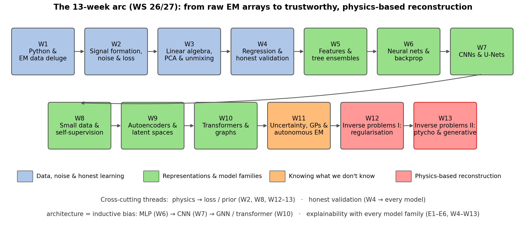
The WS 26/27 course arc: data, noise and honest learning (W1–4); representations and model families from trees to transformers (W5–10); knowing what we don’t know (W11); physics-based reconstruction (W12–13). Cross-cutting threads connect them.

• Step back and read the arc as one pipeline: represent EM data (W1–3), learn and validate honestly (W4), extract features and use strong tabular baselines (W5), build neural models with increasing inductive bias (W6 MLP → W7 CNN → W10 GNN/transformer), survive small data (W8), find latent structure (W9), quantify uncertainty and let the microscope decide (W11), and invert the physics (W12–13).
• The four threads: physics → loss/prior (W2 noise model decides the loss, W8 physics decides augmentation, W12–13 forward model decides the method); honest validation; architecture as inductive bias; explainability with every model family.
• The full pipeline a complete EM analysis contains (students can self-assess against it): (1) understand data formation — detector, dose, noise model → loss (W2), provenance (E1); (2) represent — arrays, spectra, descriptors, graphs (W1, W3, W5, W10); (3) baseline first — mean → linear → trees → NN (W4–5); (4) model with the right inductive bias (W6–10), self-supervision for small data (W8); (5) validate honestly — group splits, no leakage (W4); (6) quantify uncertainty — calibration, conformal, GPs, OOD gate (W11); (7) explain and sanity-check — attribution + intervention (W4–W10); (8) invert with the right forward model and an explicit prior (W12–13); (9) report limits.
• Do not rush this slide — it is the capstone.

The E1–E6 explainability ladder — collected over 13 weeks

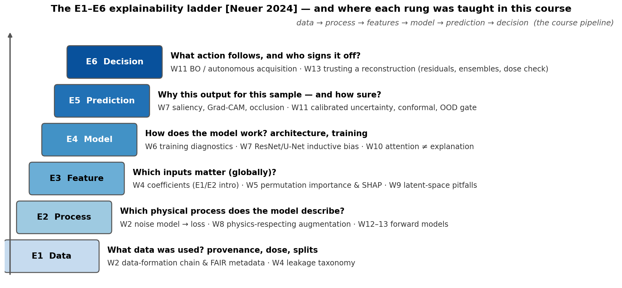
The six levels of explainability Neuer, Michael et al., (2024), ordered from data to decision, with the weeks in which each level was taught. Explainability was not a separate topic: every model family came with its own explanation tool.

• This is the synthesis of the explainability thread that ran through the whole course (W4 coefficients, W5 permutation importance/SHAP, W7 saliency/Grad-CAM/shortcut, W9 latent pitfalls, W10 attention ≠ explanation, W11 uncertainty as a trust gate). The full toolkit table is a backup slide — point students to it for revision.
• The ladder walks the same pipeline as the course: E1 data (W2/W4) → E2 process (W2/W12–13) → E3 features (W4–W5) → E4 model (W6–W10) → E5 prediction (W7/W11) → E6 decision (W11/W13). E1 and E2 are where EM scientists are strongest (provenance, physics); E3–E5 are the ML tools; E6 is where a human signs off.
• Today’s contribution is at E2 (forward models, SPA vs multislice) and E6 (should I trust this reconstruction enough to publish it?).
• Sanity-check every explanation: randomise the weights — if the saliency map does not change, it explains the image, not the model.

Recurring trust failures across the course

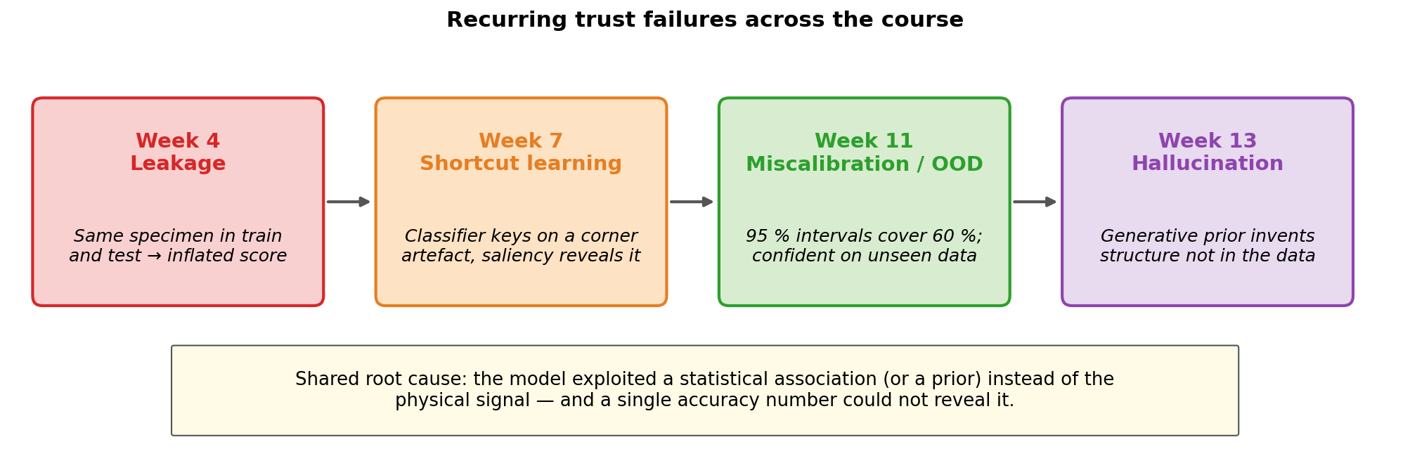
The four recurring trust failures: leakage (W4), shortcut learning (W7), miscalibration and out-of-distribution inputs (W11), hallucination (W13). All share one root cause: a statistical association or prior replaced the physical signal, and a single accuracy number could not reveal it.

• Each failure has a matching detector from the course: GroupKFold by specimen (W4), saliency + intervention (W7), reliability diagram / conformal coverage / OOD score (W11), residual + ensemble + prior-free comparison (W13).
• Ask: “Which of these would a high test accuracy have caught?” None. That is the point.

Five pillars of trustworthy EM data science

1. Correct physics: the noise model decides the loss, the forward model decides the inversion.
2. Honest validation: no leakage; group splits; report generalisation.
3. Calibrated confidence: 95 % intervals that contain the truth 95 % of the time — checked.
4. Faithful explanation: attributions verified by sanity checks and interventions.
5. Expert validation: a materials scientist checks that it makes physical sense.

• Collect the right data, build the right model, know what you don’t know, and be able to explain why you trust the answer.

• Pause on each pillar and name the week it came from: 1 → W2, W12–13; 2 → W4; 3 → W11; 4 → W5/W7; 5 → always. No tool does pillar 5 for you.
• Ask students to write down the one-sentence summary. It is the thesis of the course.
• Beyond the course (motivation, not examined): foundation models for microscopy, autonomous multi-modal acquisition, causal ML for processing, differentiable-physics reconstruction at scale.

Exam preparation

• Written exam: 60 % of the grade (miniproject 40 %); format and date as announced on the course page.
• Question types:
  • Conceptual — “When does the strong-phase approximation fail?”
  • Application — “A saliency map highlights a scale bar. What do you conclude, and which experiment confirms it?”
  • Calculation — noise model → loss, PCA/SVD, ridge/Tikhonov, backprop, GP posterior, Radon, ePIE update.
  • Judgement — “A colleague denoises a 50 e⁻/Ų image with a diffusion model trained on simulations. Three risks, one check each.”
• Study material: _shared/exam_mustknow.md. For every week: core idea in one sentence, key equation, one EM application and one failure mode.

• Calculation topics by week: noise model → loss (W2), PCA/SVD (W3), ridge/Tikhonov objective (W4/W12), backprop on a tiny graph (W6), GP posterior (W11), Fourier-slice / Radon (W12), ePIE update (W13).
• exam_mustknow.md has ≤ 10 must-know statements per week for all 13 weeks, plus the notebooks’ key numbers.
• The three-part strategy (idea, equation, application + failure mode) is the best single piece of exam advice; every must-know statement is written to support it.
• Application questions combine weeks — the most likely combinations: leakage + explainability (W4/W7), uncertainty + autonomous acquisition (W11), regularisation + hallucination (W12/13).
• Do not invent exam logistics on the spot — refer to the Week 1 slides / course page for date, duration and allowed aids.

Miniproject: final checklist

• Specification: _shared/miniproject.md — options A–E.
• Rubric (40 %): framing 15 · methodology 25 · uncertainty & validation 20 · explainability 15 · reproducibility 15 · report 10.
• Explainability with a materials conclusion; for Option D show what the prior contributes (with/without regularisation, residual plot).
• Reproducibility: jupyter nbconvert --to notebook --execute your_notebook.ipynb must run end-to-end.

• Options: A segmentation, B spectral unmixing & clustering, C property regression, D small imaging inverse problem, E atom-column descriptors & defect classification.
• Explainability examples: Grad-CAM on a failure case (A), NMF endmembers as interpretable spectra (B), SHAP on descriptors (C/E). Uncertainty: calibrated intervals, reliability diagram or posterior/ensemble spread; honest group splits.
• Option D directly uses Weeks 12–13: a deblurring, tomography or small ptychography problem. The strongest submissions show the λ trade-off (U-curve) and discuss what the prior may have invented.
• Action item: “open miniproject.md tonight and check your notebook against the rubric rows”.

Self-study notebook

• Notebook: notebooks/week13_ptychography.ipynb —
• Parts 1–5: forward model → ePIE (0.0991 → 0.0021); overlap sweep 4 / 6 / 8 px → 0.0021 / 0.0067 / 0.0091.
• Part 6: autodiff gradient descent with \(O=e^{i\phi}\) — \(8.7\times10^{-5}\) vs \(7.7\times10^{-4}\) (ePIE) after 200 passes.
• Part 7: 100 e⁻/pattern, TV prior in one line; find the best \(\lambda_{TV}\) and explain the U-curve.
• CPU only, < 1 min.

• Parts 1–4: synthetic phase object and probe → forward model → ePIE. Part 5 is exercise 1 (overlap sweep). Part 6 aligned phase error 2.9e-4 rad vs 1.7e-3 rad for ePIE. Part 7 is exercise 2.
• Point students to the two questions in exercise 2 about early stopping and dose — both are exam-style.
• Try next: add a probe update, or the Poisson NLL instead of the amplitude loss. For the curious: extend forward_torch to two slices with a Fresnel propagator between them — a two-slice multislice model is ~5 extra lines.

Summary

• Ptychography: overlap makes phase retrieval over-determined; ePIE solves it by alternating projections.
• Object physics: weak phase → strong phase → multislice for thick samples; depth has a missing wedge; thermal vibrations set the final limit.
• Autodiff gradient descent solves the same loss with any parameters, losses and priors.
• Generative priors: GANs → diffusion (stable, diverse, gives a score); DPS adds a data-consistency gradient through Tweedie’s estimate.
• Physics constraints: soft (loss) vs hard (parameterisation); wrong physics biases confidently.
• Trust: low dose = strong prior = hallucination risk — residuals, ensembles, prior-free baselines.
• Synthesis: E1–E6 ladder and five pillars — more powerful = more assumptions.

• One sentence per bullet; this is the slide to photograph before the exam.

Must-know takeaways (Week 13)

1. Detectors record \(|\psi|^2\); ptychographic overlap makes phase retrieval over-determined: \(I_j = |\mathcal{F}[P\cdot O(\mathbf{r}-\mathbf{r}_j)]|^2\).
2. ePIE: replace the Fourier amplitude with \(\sqrt{I_j}\), back-transform, update \(O_j \mathrel{+}= \beta\,P^*/|P|^2_{\max}\,(\psi'_j-\psi_j)\).
3. SPA: \(\psi_{\text{exit}} = \psi_0\,e^{i\sigma V_p}\); fails for thick samples / strong scatterers → multislice (transmit, propagate, repeat).
4. Ptychography = loss minimisation; autodiff differentiates through FFT and modulus, so probe, positions, slices and priors are just extra terms.
5. Posterior score = prior score + likelihood score; DPS approximates the likelihood at the Tweedie estimate \(\hat{\mathbf{x}}_0\).
6. Hard constraints (parameterisation) are exact but only as good as their physics; soft constraints need a λ.
7. The weaker the data, the more the prior decides — check residuals, ensembles and a prior-free baseline before trusting a generative reconstruction.

• These mirror _shared/mustknow_parts/week13.md (which has the full ten statements, including the E1–E6 ladder, causality and the five pillars).

Closing

• Over 13 weeks you built a data-science toolkit for EM — from noise models, trees, CNNs, transformers and GPs to physics-based and generative reconstruction.
• The scientific obligation: you are responsible for validating every number, explanation and reconstruction against physics.
• Next steps: exam_mustknow.md, miniproject.md, and the Ai4Mat companion notebooks.
• Thank you for 13 weeks of work.

• Deliver without rushing; the last lecture deserves a moment. The tools do not absolve the scientist.
• “You are now equipped to contribute to the next generation of intelligent electron microscopy.”
• Every student in this room will meet a model that looks right and is wrong. Catching it — validation, explanation, physics — is what this course was for.

Continue

• ← Previous: Unit 12 — Inverse problems I: regularisation, tomography & sensor fusion
• All courses

Backup slides

Material that did not fit the 90-minute lecture path — for self-study and questions.

Beyond one view: ptychographic tomography

• Combine Week 12 and Week 13: reconstruct a phase projection (or multislice stack) at every tilt angle, then solve a tomography problem — or do both at once.
• Ptychographic atomic electron tomography: 34.5 million diffraction patterns → atomic-resolution tilt series of a double-wall carbon nanotube with an encapsulated ZrTe structure; revealed a previously unobserved ZrTe₂ phase. Pelz, Philipp M. et al., (2023), doi:10.1038/s41467-023-43634-z
• Multislice ptychographic tomography: 2 Å axial and 0.7 Å lateral resolution in a volume beyond the depth-of-field limit — a 13.5× axial improvement over single-view multislice. Romanov, Andrey et al., (2024), doi:10.1088/2515-7639/ad9ad2
• End-to-end: reconstruct the 3-D potential directly from the unaligned 4D-STEM tilt series, including alignment and a restricted tilt range — sub-Å near-isotropic resolution. You, Shengbo et al., (2024), doi:10.1088/1402-4896/ad9a1a
• Why this became possible: all of these are one big differentiable forward model optimised by gradient descent.

• These are our own group’s papers — use them as “this is what the inverse-problem toolbox of Weeks 12–13 does in current research”.
• Pelz et al. 2023: light elements (C) and heavy elements (Zr, Te) are imaged together in 3-D — HAADF tomography cannot do this because C is invisible next to Te.
• End-to-end: nuisance parameters (tilt-axis alignment, probe, positions) are optimised jointly with the volume. “Everything is a parameter; autodiff gives the gradient.”

What ptychography buys: dose–resolution trade-off

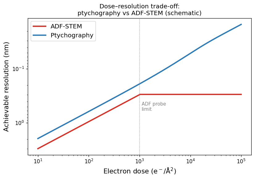
Schematic dose–resolution trade-off for ADF-STEM (red) and ptychography (blue); y-axis inverted (higher = finer). In the low-dose regime both scale as \(d \propto 1/\sqrt{\text{dose}}\), but ptychography uses all scattered electrons and achieves better resolution at equal dose. At high dose ADF saturates at the probe-size limit; ptychography keeps improving because it deconvolves the probe. Chen, Zhen et al., (2021), doi:10.1126/science.abg2533

• Low dose: both limited by Poisson noise, \(1/\sqrt{N}\) scaling. Ptychography uses the whole diffraction pattern instead of a high-angle annulus.
• High dose: ADF is limited by the probe (hardware); ptychography recovers information beyond the probe size because the diffraction pattern encodes sub-probe structure.
• Practical: for beam-sensitive materials (MOFs, zeolites, 2-D materials, biological samples) dose efficiency is the reason to use ptychography.

Experimental parameters and quality control

• What you choose: probe size / defocus (aberration corrector settings), scan step (~20–40 % of the probe diameter), camera length (detector angular range ↔︎ real-space pixel size), total dose.
• Detector sampling: the diffraction pattern must be Nyquist-sampled; under-sampling aliases (Week 2).
• Partial coherence: model as mixed probe states, \(I_j = \sum_k |\mathcal{F}[P_k \cdot O_j]|^2\) — trivial to add in an autodiff framework.
• What you get: complex object \(O(\mathbf{r})\) (amplitude + phase), reconstructed probe(s), refined positions.
• Quality check: amplitude error decreasing smoothly and plateauing well below its start; residual consistent with Poisson noise; reconstruction stable across initialisations and data halves (a half-set comparison, like cryo-EM FSC). Maiden, Andrew M. et al., (2009), doi:10.1016/j.ultramic.2009.05.012

• In the notebook, step 4 px on a 16 px probe = 25 % of the probe diameter = 75 % overlap.
• Half-set comparison: reconstruct from odd and even scan positions separately, compare in Fourier space; frequencies where they agree are supported by the data. This is an honest-validation idea (Week 4) applied to reconstruction.

The plug-and-play framework: any denoiser as a prior

• Insight: the proximal step of a regulariser \(R\) has the same form as Gaussian denoising. Kamilov, Ulugbek S. et al., (2023), doi:10.1109/MSP.2022.3199595
• Plug-and-play (PnP): replace the proximal step in ADMM / proximal gradient descent with any strong denoiser — BM3D, a DnCNN or a U-Net (Week 7) trained on EM images.
• Algorithm: alternate
  1. Data step: \(\mathbf{x} \leftarrow \mathbf{x} - \eta \nabla_{\mathbf{x}} \|H(\mathbf{x}) - \mathbf{y}\|^2\)
  2. Prior step: \(\mathbf{x} \leftarrow D_\sigma(\mathbf{x})\) (apply the learned denoiser)
• Result: the denoiser defines the prior implicitly. Diffusion models are the logical extreme: a denoiser trained at every noise level.

• Recap of Week 12 PnP, with the forward pointer to diffusion: a diffusion model is a stack of denoisers \(D_\sigma\) for all \(\sigma\), and Tweedie’s formula turns a denoiser into a score. That is why DPS looks like PnP with a noise schedule.
• Convergence guarantees need contractive denoisers, which most networks are not exactly — in practice it usually works. Not examined.

Tweedie’s formula: a denoiser gives a clean-image estimate

• At any step \(t\) the network gives an estimate of the clean image (Tweedie): \[\hat{\mathbf{x}}_0(\mathbf{x}_t) = \frac{\mathbf{x}_t + (1-\bar\alpha_t)\,\nabla_{\mathbf{x}_t}\log p_t(\mathbf{x}_t)}{\sqrt{\bar\alpha_t}} = \frac{\mathbf{x}_t - \sqrt{1-\bar\alpha_t}\,\boldsymbol\epsilon_\theta(\mathbf{x}_t,t)}{\sqrt{\bar\alpha_t}}\]
• \(\hat{\mathbf{x}}_0\) is the posterior mean \(\mathbb{E}[\mathbf{x}_0 \mid \mathbf{x}_t]\) — blurry early (large \(t\)), sharp late.
• Why this matters for inverse problems: we can push \(\hat{\mathbf{x}}_0\) through the physical forward model \(H\) at every step and compare with the measurement \(\mathbf{y}\) — even though \(\mathbf{x}_t\) itself is noisy.
• This is the one ingredient that turns an unconditional generator into a reconstruction algorithm.

• Tweedie’s formula is the key technical step of diffusion posterior sampling. Present it as “the network’s best guess of the clean image, given the noisy one”.
• Early in sampling \(\hat{\mathbf{x}}_0\) is an average over many plausible images (blurry); late it commits to one.

Generative models for EM: applications

• Denoising at low dose: learned priors preserve atomic contrast far better than BM3D/NLM at extreme noise; self-supervised training (Noise2Void / blind-spot) avoids paired clean data.
• Super-resolution & inpainting: fill in sub-sampled scans (dose reduction by sparse scanning, compressed sensing) — conditioned on measured pixels.
• Reconstruction priors: diffusion/PnP priors inside ptychography and tomography — especially to fill the missing wedge.
• Synthetic training data & inverse design: generate realistic micrographs for training segmentation (Weeks 7–8) and crystal/microstructure candidates (MG Unit 12).
• The common question in every case: did the network reveal structure or invent it? Low dose = weak likelihood = strong prior = high risk.

• Denoising is the most widely adopted application because it directly addresses dose. The risk: “looks better” but removes real disorder or beam damage.
• Missing-wedge inpainting with learned priors is an active research area in tomography — directly continues Week 12.

Choosing a reconstruction method

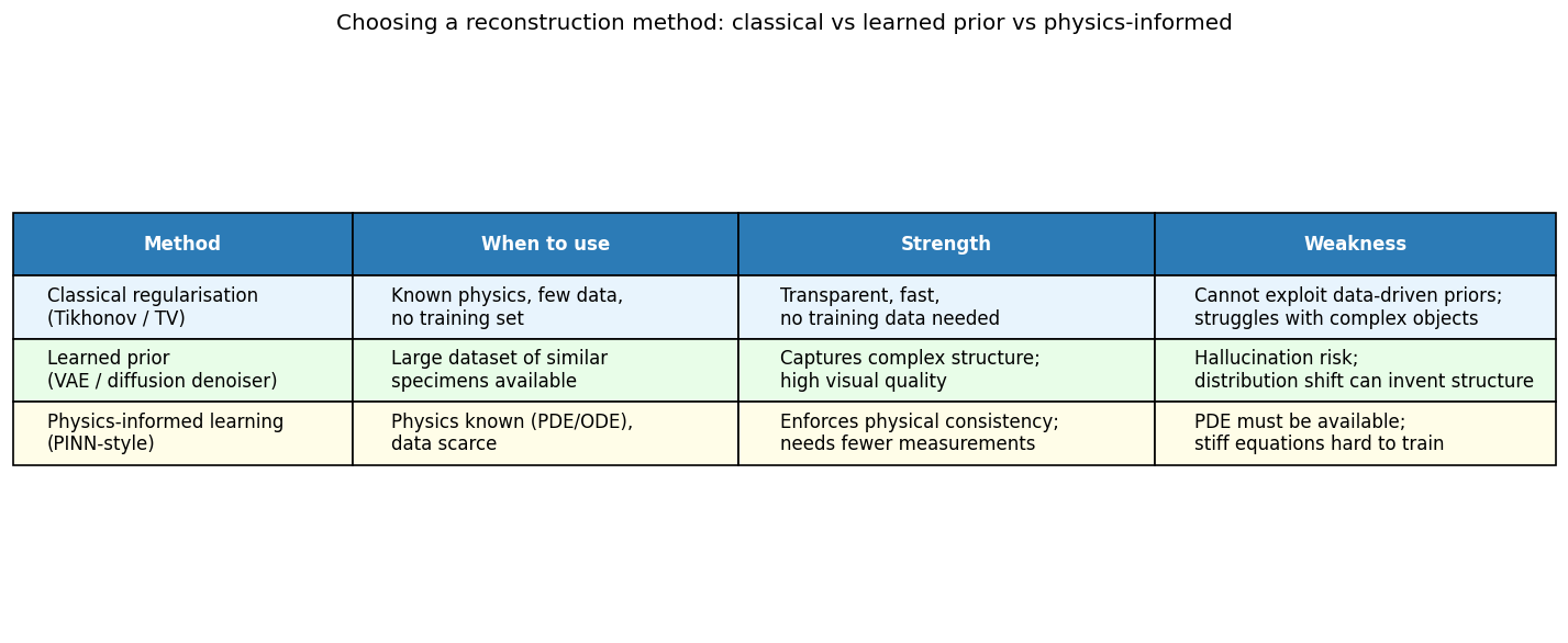
Decision table: classical regularisation (Tikhonov/TV) for well-understood physics and limited data; learned priors (GAN/diffusion) when a large dataset of similar specimens exists; physics-informed learning when governing equations are known and data are scarce. Combinations (physics + learned prior, e.g. DPS with a physical forward model) are the active research direction.

• Row 1: default for new or unusual specimens — no training data needed, predictable failure (smoothing bias).
• Row 2: high performance when curated in-distribution training data exist; subtle failure modes.
• Row 3: physics known, data scarce — e.g. multislice ptychography with the multislice model as forward operator.
• Practical ordering: always run a classical baseline first (Week 5 baseline ladder, applied to reconstruction).

The explainability & trust toolkit at a glance

Method	Question it answers	Works on	Week
Coefficients / partial dependence	How does the output change with a feature?	Linear / additive models	W4
Permutation importance, SHAP Lundberg, Scott M. et al., (2017)	Which features matter, globally and per sample?	Any model	W5
Saliency, Grad-CAM Selvaraju, Ramprasaath R. et al., (2017), occlusion	Which pixels drove this prediction?	CNNs (occlusion: any)	W7
Latent-space maps, t-SNE/UMAP	What structure did the model find? (beware distances)	AEs / VAEs / embeddings	W9
Attention maps	Where did the transformer look? (≠ why)	Transformers	W10
Calibration, conformal, OOD gate	How sure — and is this input in-distribution?	Any predictor	W11
Residuals, posterior ensembles, half-sets	Is this reconstruction supported by the data?	Inverse problems	W12–13

• Sanity check every explanation — e.g. randomise the weights: if the saliency map does not change, it explains the image, not the model. Adebayo, Julius et al., (2018)

• Reference slide — students should photograph it. Every row is examinable at the “what does it answer, what does it need” level.
• The “Works on” column: gradient methods need differentiability (no random forest, no black-box simulator); permutation importance and occlusion are model-agnostic.
• The last row is today’s addition: for reconstructions, the explanation is the residual and the ensemble — “which parts of the output are forced by the data?”.

References

Hard-x-ray lensless imaging of extended objects, Physical Review Letters, John M. Rodenburg, A. C. Hurst, A. G. Cullis, B. R. Dobson, F. Pfeiffer, O. Bunk, C. David, K. Jefimovs, & I. Johnson https://doi.org/10.1103/PhysRevLett.98.034801.

An improved ptychographical phase retrieval algorithm for diffractive imaging, Ultramicroscopy, Andrew M. Maiden & John M. Rodenburg https://doi.org/10.1016/j.ultramic.2009.05.012.

The scattering of electrons by atoms and crystals. I. A new theoretical approach, Acta Crystallographica, J. M. Cowley & A. F. Moodie https://doi.org/10.1107/S0365110X57002194.

Ptychographic transmission microscopy in three dimensions using a multi-slice approach, Journal of the Optical Society of America A, Andrew M. Maiden, Martin J. Humphry, & John M. Rodenburg https://doi.org/10.1364/JOSAA.29.001606.

Electron ptychography achieves atomic-resolution limits set by lattice vibrations, Science, Zhen Chen, Michal Odstrcil, Yi Jiang, Yimo Han, Ming-Hui Chiu, Lain-Jong Li, & David A. Muller https://doi.org/10.1126/science.abg2533.

Using automatic differentiation as a general framework for ptychographic reconstruction, Optics Express, Saugat Kandel, Siddharth Maddali, Marc Allain, Stephan O. Hruszkewycz, Chris Jacobsen, & Youssef S. G. Nashed https://doi.org/10.1364/OE.27.018653.

A plug-and-play image reconstruction framework, IEEE Signal Processing Magazine, Ulugbek S. Kamilov, Charles A. Bouman, Gregery T. Buzzard, & Brendt Wohlberg https://doi.org/10.1109/MSP.2022.3199595.

Generative adversarial nets, Advances in neural information processing systems, Ian Goodfellow, Jean Pouget-Abadie, Mehdi Mirza, Bing Xu, David Warde-Farley, Sherjil Ozair, Aaron Courville, & Yoshua Bengio.

Score-based generative modeling through stochastic differential equations, International conference on learning representations (ICLR), Yang Song, Jascha Sohl-Dickstein, Diederik P. Kingma, Abhishek Kumar, Stefano Ermon, & Ben Poole.

Denoising diffusion probabilistic models, Advances in neural information processing systems, Jonathan Ho, Ajay Jain, & Pieter Abbeel.

Diffusion posterior sampling for general noisy inverse problems, International conference on learning representations (ICLR), Hyungjin Chung, Jeongsol Kim, Michael T. Mccann, Marc L. Klasky, & Jong Chul Ye.

Physics-informed neural networks: A deep learning framework for solving forward and inverse problems involving nonlinear partial differential equations, Journal of Computational Physics, Maziar Raissi, Paris Perdikaris, & George E. Karniadakis https://doi.org/10.1016/j.jcp.2018.10.045.

Artificial neural networks for solving ordinary and partial differential equations, IEEE Transactions on Neural Networks, Isaac G. Lagaris, Aristidis Likas, & Dimitrios I. Fotiadis.

Solving complex nanostructures with ptychographic atomic electron tomography, Nature Communications, Philipp M. Pelz, Sinéad M. Griffin, Scott Stonemeyer, Derek Popple, Hannah DeVyldere, Peter Ercius, Alex Zettl, Mary C. Scott, & Colin Ophus https://doi.org/10.1038/s41467-023-43634-z.

Machine learning for engineers: Introduction to physics-informed, explainable learning methods for AI in engineering applications, Michael Neuer & others.

Multi-slice electron ptychographic tomography for three-dimensional phase-contrast microscopy beyond the depth of focus limits, Journal of Physics: Materials, Andrey Romanov, Min Gee Cho, Mary Cooper Scott, & Philipp Pelz https://doi.org/10.1088/2515-7639/ad9ad2.

Near-isotropic sub-Ångstrom 3d resolution phase contrast imaging achieved by end-to-end ptychographic electron tomography, Physica Scripta, Shengbo You, Andrey Romanov, & Philipp M. Pelz https://doi.org/10.1088/1402-4896/ad9a1a.

A unified approach to interpreting model predictions, Advances in neural information processing systems, Scott M. Lundberg & Su-In Lee.

Grad-CAM: Visual explanations from deep networks via gradient-based localization, Proceedings of the IEEE international conference on computer vision, Ramprasaath R. Selvaraju, Michael Cogswell, Abhishek Das, Ramakrishna Vedantam, Devi Parikh, & Dhruv Batra.

Sanity checks for saliency maps, Advances in neural information processing systems (NeurIPS), Julius Adebayo, Justin Gilmer, Michael Muelly, Ian Goodfellow, Moritz Hardt, & Been Kim.