Materials Genomics
Unit 6: Local Atomic Environments & Universal MLIPs
FAU Erlangen-Nürnberg


§0 · Frame
01. Today’s question
How do we hand a crystal to a regression model?
- A crystal is positions, species, and a periodic cell — not a vector.
- Some properties are dictated by what is in the formula; others by where the atoms sit; others still by who sits next to whom.
- A representation that ignores any one of these layers will fail on whichever properties depend on that layer.
Today’s claim.
- There is a ladder of structural descriptors, from formula-only Magpie vectors to atom-centred SOAP / ACSF.
- Climbing the ladder costs computation and interpretability; not climbing it costs accuracy on motif-sensitive targets.
- The art of materials-genomics representation is knowing where on the ladder a given problem belongs.
02. Where we are
Recap — what we already have
- Unit 1–4: quantum mechanics, electronic structure, MD/MC. Atomistic structure is the physics.
- Unit 5: Monte Carlo sampling and continuum mechanics — the simulation side of the data pipeline.
- MFML W5: clustering & autoencoders — first hint of learned representations.
- ML-PC W2: PCA / SVD as the linear unsupervised baseline.
Forward pointer
- Unit 7 (in two weeks): crystals as graphs — GNNs as the learned analogue of today’s fixed-aggregation descriptors.
Today — Unit 6 in one line
- Hand-engineered atom-centred descriptors as a complement (and competitor) to learned graph representations.
- Five chunks: composition baselines, locality discipline, simple geometry, ACSF + SOAP, pooling.
- Closes with failure modes — the difference between pipelines that work and pipelines that publish but don’t reproduce.
03. Learning outcomes
By the end of 90 minutes, you can:
- Place a problem on the descriptor ladder — composition, globally-pooled, atom-centred, or learned graph — and justify the choice.
- Compute a Magpie / matminer baseline and report it before any structure-aware model.
- Construct a local atomic environment under periodic boundary conditions, with attention to the cutoff and to invariance.
- Distinguish coordination, bond-length, bond-angle, and Voronoi descriptors by what they preserve and what they discard.
- Explain ACSF and SOAP at the operational level — what each function asks the neighbourhood, why it is invariant, and where the cost sits.
- Choose a pooling rule (mean, histogram, species-resolved) consistent with the scientific mechanism of the target.
- Diagnose a descriptor pipeline for cutoff sensitivity, periodic-image bugs, polymorph aliasing, and long-range physics limits.
- Articulate when a local descriptor is the wrong tool and what to reach for instead.
§A · The descriptor ladder
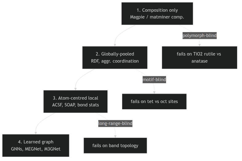
04. The descriptor ladder
Four tiers of structural descriptor
- Composition only — Magpie / matminer composition statistics. Formula in, vector out. No structure used.
- Globally-pooled structural — RDF, partial RDF, structure-aggregated coordination. Uses positions, averages over the cell.
- Atom-centred local — ACSF, SOAP, bond geometry. One vector per site, then pooled.
- Learned graph — GNNs (Unit 7). The aggregation itself is learned.
05. Tier 1 — Magpie elemental statistics (Ward et al. 2016)
The construction
- Take the chemical formula; for each element, look up per-element properties (atomic number, mass, electronegativity, atomic radius, valence-electron count, group, period, melting point, ionic radii, …).
- Compute element-wise statistics across the formula:
- mean, weighted mean, min, max, range, standard deviation.
- Concatenate into a fixed-length vector (≈ 40–60 numbers for typical setups).
Worked example: \(\mathrm{Li}_x \mathrm{Ni}_y \mathrm{Co}_z \mathrm{Mn}_w \mathrm{O}_2\)
- Stoichiometric weights \(\{x, y, z, w, 2\}\).
- For each per-element scalar (e.g. electronegativity), report
{wmean, wstd, range, max, min}. - The output is the same shape regardless of how many elements the formula has.
- Cheap, interpretable, scale-invariant — a baseline you can compute on a laptop in milliseconds.
06. Tier 1 — The matminer feature library (Ward et al. 2018)
What matminer adds on top of Magpie
- A library of feature generators, each with a clear interface:
ElementProperty(Magpie itself, plus alternative tables: Deml, Pymatgen, Slater).OxidationStates,IonProperty,BandCenter,Stoichiometry.- Structure-aware generators (when a
Structureobject is supplied): coordination statistics, bond fractions, X-ray diffraction patterns, …
- Standard-conforming: every featuriser exposes
feature_labels()and afeaturize(...)API.
Why matminer is the tier-1 working tool
- Reproducibility: papers report a named featuriser stack, not bespoke code.
- Composability:
MultipleFeaturizer([...])stacks generators into one feature matrix. - Interpretability: feature names like
MagpieData mean Electronegativitysurvive into SHAP plots and feature-importance tables. - Scaling: parallelisation built in; pandas-native.
07. Why composition-only is stronger than it should be
The empirical picture
- On many bulk-property tasks (formation energy, band gap, bulk modulus), Magpie + random forest reaches within ~5–10% of the best structure-aware model.
- For datasets ≲ 10 000 examples, the gap is often zero.
- Composition-only models train in seconds and ship in production.
Why it works
- Property-determining chemistry is dominated by element identity and stoichiometry; structure is a refinement, not a first-order signal.
- Bulk thermodynamic targets are spatially averaged by definition — they integrate over local detail.
- The chemical periodicity that Magpie captures (group, period, valence) carries a lot of the variance in the data.
The pedagogical lesson, said aloud: every materials-ML project should report a composition-only baseline before any structure-aware model. If structure cannot beat composition, the bottleneck is the data, the target, or the split — not the representation.
08. Where composition-only fails
Polymorph blindness
- \(\mathrm{TiO}_2\) exists as rutile (tetragonal, \(E_g \approx 3.0\,\mathrm{eV}\)), anatase (tetragonal, \(E_g \approx 3.2\,\mathrm{eV}\)), and brookite (orthorhombic).
- All three share the formula \(\mathrm{TiO}_2\); their Magpie vectors are identical.
- A composition-only model cannot resolve which polymorph a sample is.
Defects, doping, disorder
- Pristine vs vacancy-rich \(\mathrm{Li}_x\mathrm{CoO}_2\): same formula range, very different ionic-conductivity behaviour.
- Ordered vs disordered alloys: same composition, different mixing entropy and band structure.
- Composition collapses all of these to a single point.
Decision rule. If the science depends on which polymorph, which defect, or how an alloy is ordered — composition alone is the wrong tool. Climb the ladder.
09. Tier 2 — Radial distribution functions
The total RDF \(g(r)\)
- Probability of finding any atom at distance \(r\) from a reference atom, normalised by an ideal-gas reference: \[ g(r) = \frac{V}{N^2}\,\Big\langle \sum_{i \neq j} \delta(r - r_{ij}) \Big\rangle. \]
- Captures isotropic structure: peak positions = coordination shells, peak widths = thermal / static disorder.
The partial RDF \(g_{AB}(r)\)
- Restrict the pair to species \(A\) and \(B\): \[ g_{AB}(r) \propto \big\langle \sum_{i \in A,\, j \in B,\, i \neq j} \delta(r - r_{ij}) \big\rangle. \]
- Recovers chemistry that the total RDF and Magpie vectors lose.
- For an \(n\)-element compound: \(\binom{n+1}{2}\) partial RDFs.
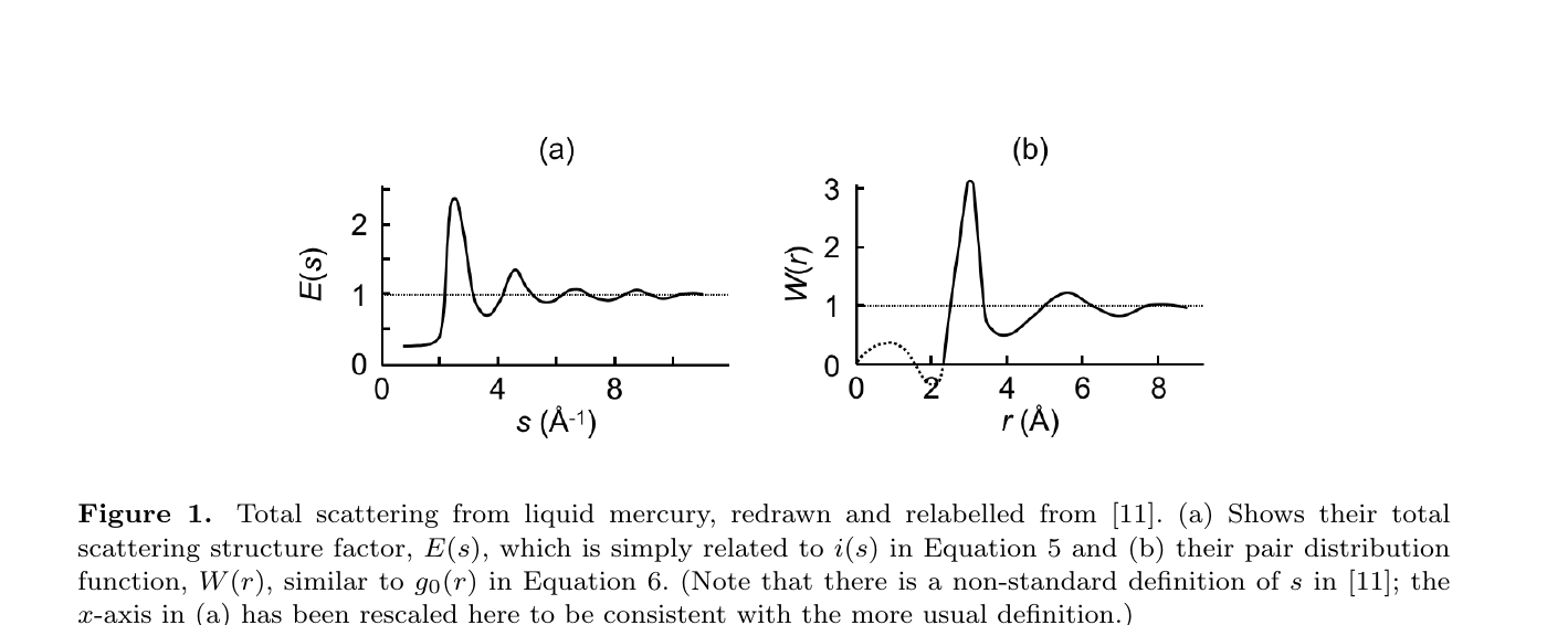
09b. The RDF is an experimental observable — PDF analysis & neutron total scattering
PDF analysis: structure factor ↔︎ \(g(r)\)
- A diffraction experiment measures the total scattering structure factor \(S(Q)\) — Bragg + diffuse, in one shot.
- A sine Fourier transform gives the pair distribution function \(G(r)\) — the experimentally-measured RDF: \[ G(r) = \frac{2}{\pi}\!\int_0^{\infty}\! Q\,[S(Q)-1]\sin(Qr)\,\mathrm{d}Q. \]
- Peaks = neighbour shells, widths = disorder — exactly the \(g(r)\) of slide 09, now an observable (Keen 2020).
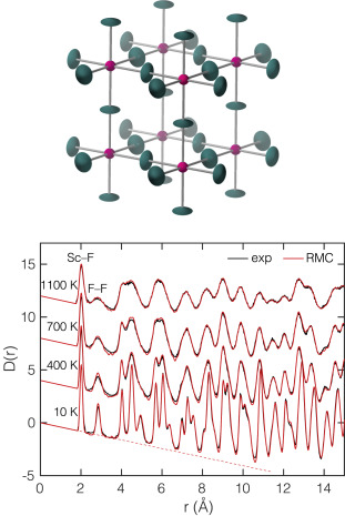
Neutrons measure it directly
- Neutrons scatter from nuclei → flat form factor (large \(Q_{\max}\) → sharp \(r\)-resolution), isotope/light-element contrast, no electronic falloff.
- Total scattering at spallation sources captures Bragg and diffuse → a snapshot of the local structure, not just the average crystal.
- Refine with reverse Monte Carlo / big-box modelling to recover an atomistic ensemble consistent with the measured \(G(r)\) (Dove and Li 2022).
Note
The Tier-2 RDF descriptor is not arbitrary: it is a quantity you can measure. Models trained on simulated \(g(r)\) can be validated against an experimental PDF, and experimental PDFs can be featurised on the same grid.
10. Tier 2 — Structure-aggregated coordination (Ward et al. 2017)
The descriptors
- Per-element-pair coordination number, averaged over sites: \(\langle N_{AB} \rangle\).
- Bond-length statistics per pair: \(\langle r_{AB} \rangle\), \(\sigma_{r_{AB}}\).
- Bond-angle moments per triplet: mean angle, variance, skewness.
- matminer:
SiteStatsFingerprint,BondFractions,CrystalNNFingerprint.
What this rung gains over the RDF
- Species-resolved by construction (the partial RDF is the integral; this is the moment summary).
- Dimensionally compact: a few moments per pair, not a histogram.
- Easier to feed into linear/tree-based models; no large
n_binsaxis.
What it still discards
- Per-site identity (it averages over sites, like the RDF).
- Higher-order angular correlations beyond the moment summary.
11. Why we now go local — the motif argument
The recurring failure mode of tiers 1 and 2
- A target controlled by a minority motif (defects, dopant sites, surface terminations, intercalation sites).
- Tiers 1 and 2 average that motif away — its signal becomes a small perturbation to a large mean.
- A model trained on tier 1/2 features therefore cannot see the motif, no matter how much capacity you add.
The motif argument
- A local descriptor is computed at each atomic site, then optionally pooled.
- Pooling is a choice, not a default: you can keep the distribution.
- A defect site stops being a perturbation to the mean and becomes a tail of the descriptor distribution.
- That is what makes locality earn its keep.
The right question to ask of any descriptor: if the property of interest depends on a motif present at 1% of sites, does the descriptor preserve the 1% motif, or average it into the 99%? Tiers 1–2 average; tier 3 preserves.
12. The ladder, restated as a decision tree
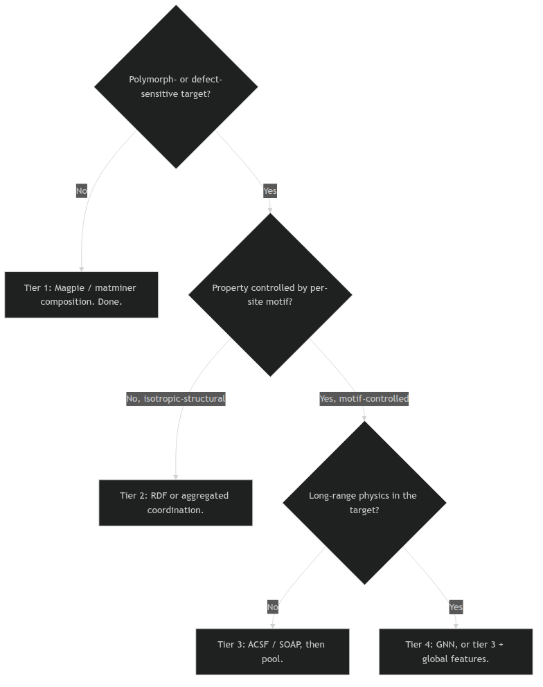
Descriptor decision tree
§B · What is a local atomic environment
13. Definition: the local environment of atom \(i\)
The objects we keep
For atom \(i\) at position \(\mathbf{r}_i\) with species \(Z_i\):
- the central species \(Z_i\),
- the neighbouring species \(\{Z_j\}_{j \in \mathcal{N}(i)}\),
- the relative positions \(\{\mathbf{r}_j - \mathbf{r}_i\}_{j \in \mathcal{N}(i)}\),
- and (optionally) angles \(\theta_{jik}\) between neighbour pairs.
We deliberately do not keep the absolute position of \(i\) in the cell.
Two ways to define \(\mathcal{N}(i)\)
- Radial cutoff: \(\mathcal{N}(i) = \{j : 0 < r_{ij} < r_c\}\). One scalar parameter.
- Voronoi tessellation: \(j \in \mathcal{N}(i)\) iff Voronoi cells of \(i\) and \(j\) share a face (optionally with a face-area threshold). No cutoff parameter, but face-area thresholds reintroduce one.
14. Neighbour construction under a radial cutoff
The formula and the count
- Indicator definition: \(j \in \mathcal{N}_{r_c}(i) \iff 0 < r_{ij} < r_c\).
- Coordination number: \[ N_i(r_c) = \sum_{j \neq i} \mathbb{1}[r_{ij} < r_c]. \]
- \(N_i\) is a step function in \(r_c\) — every shell adds a jump.
Smooth cutoffs
- A hard cutoff is non-differentiable in atomic positions.
- ACSF and SOAP therefore multiply by a smooth window: \[ f_c(r) = \begin{cases} \tfrac{1}{2}\left[\cos\!\left(\tfrac{\pi r}{r_c}\right) + 1\right] & r < r_c, \\ 0 & r \geq r_c. \end{cases} \]
- Smooth cutoffs are required for descriptors used in machine-learned interatomic potentials.
15. Periodic images are not optional
The geometry
- A crystal is described by a fundamental cell + lattice vectors \(\{\mathbf{a}_1, \mathbf{a}_2, \mathbf{a}_3\}\).
- Atom \(i\) has images at \(\mathbf{r}_i + n_1 \mathbf{a}_1 + n_2 \mathbf{a}_2 + n_3 \mathbf{a}_3\) for all \(\mathbf{n} \in \mathbb{Z}^3\).
- The “true” neighbour list of atom \(i\) at the cell centre and at the cell boundary must be physically equivalent.
The trap and the fix
- Trap: compute neighbours from atomic coordinates inside the unit cell only; atoms near the boundary acquire fake low coordination.
- Fix: enumerate images \((n_1, n_2, n_3)\) within \(\mathbf{n}\) such that the image distance \(\le r_c\), and include image atoms in the neighbour search.
- Standard tools: ASE
NeighborList, pymatgenStructure.get_neighbors, MDAnalysisdistance_array(box=...). Use them.
The first audit on any local-descriptor pipeline: plot the coordination number for ten boundary atoms and ten interior atoms, check that they look chemically equivalent. If they don’t, the periodic images are wrong, not the descriptor.
16. Invariance discipline — what a descriptor must respect
A useful local descriptor \(\phi(\text{environment of } i)\) must satisfy:
- Translation invariance. Shift the crystal by any \(\mathbf{t}\): \(\phi\) unchanged.
- Rotation invariance (or equivariance). Rotate by any \(R \in SO(3)\): \(\phi\) either unchanged (invariant) or transforms predictably (equivariant).
- Permutation invariance. Reorder identical neighbours: \(\phi\) unchanged.
- Continuity. Small displacement \(\delta \mathbf{r}_j\): small change \(\delta \phi\) — no jumps.
- Chemical sensitivity. Replace \(Z_j\) with a chemically distinct \(Z_j'\): \(\phi\) must change.
If a descriptor fails any of these, the model learns file conventions or noise instead of physical structure. Invariance is not pedantry — it is the difference between a descriptor that generalises and a descriptor that overfits to coordinate-system accidents.
17. Why raw Cartesian coordinates are the wrong baseline
Three failures, in one slide
- Origin dependence: translating the crystal changes every input but no chemistry.
- Orientation dependence: rotating the cell changes every input but no chemistry.
- Atom-ordering dependence: the same crystal written with two atom orderings produces two different inputs.
A regression model fed raw Cartesians has to learn all three invariances from the data — which it almost never does cleanly, especially with small materials datasets.
The “data augmentation will save us” objection
- Adding rotated copies as augmentation forces the model to approximately learn rotation invariance.
- For small datasets, this is wasteful: invariance can be built in (descriptor) instead of fit (model capacity).
- For very large datasets and large models, the augmentation route is increasingly competitive — see equivariant GNNs and end-to-end learned descriptors.
- Today’s lecture is about the small-data, hand-built end of the spectrum.
18. The local-environment object, fully written out
The mathematical object
For atom \(i\), the local environment is the set \[ \mathcal{E}_i = \{(Z_j,\, \mathbf{r}_j - \mathbf{r}_i) : j \in \mathcal{N}(i)\}, \] plus the central species \(Z_i\) and (optionally) the cell metric.
The descriptor \(\phi\) is any function \(\mathcal{E}_i \mapsto \mathbb{R}^d\) that respects the five invariances of slide 16.
The taxonomy of \(\phi\)
- Counting: coordination number (\(d = 1\)). Loses geometry.
- Histograms: binned bond lengths and angles (\(d \approx 50\)). Loses higher-order shape.
- ACSF: designed radial + angular functions (\(d \approx 100\text{–}1000\)). Hand-engineered, interpretable.
- SOAP: smooth density + spherical-harmonic expansion (\(d \approx 500\text{–}5000\)). Systematic, expressive.
- Equivariant features: vector-/tensor-valued \(\phi\), beyond today’s scope.
19. Cutoff radius as a scientific hyperparameter
\(r_c\) is part of the model
- \(r_c\) too small → first or second coordination shell missing → chemistry truncated.
- \(r_c\) too large → expensive, mixes local chemistry with weakly relevant structure.
- \(r_c\) chosen to match a physically meaningful length (first-shell, second-shell, magnetic exchange, screening length) is most defensible.
Heuristics, not formulas
- For metals and metallic glasses: \(r_c \approx 6\)–\(8\) Å covers two coordination shells.
- For oxides: \(r_c \approx 5\)–\(6\) Å covers cation–anion–cation paths.
- For molecular crystals: \(r_c \approx 4\)–\(5\) Å covers nearest molecules.
- Always run a sensitivity scan; if results swing wildly with \(r_c\), the descriptor is too brittle for the problem.
§C · Simple geometric local descriptors
20. Coordination number — the simplest summary
Per-atom coordination
\[ N_i(r_c) = \sum_{j \neq i} \mathbb{1}[r_{ij} < r_c]. \]
- One scalar per atom: cheap, interpretable.
- Resolves the most common motif families:
- \(N_i = 4\): tetrahedral, square-planar.
- \(N_i = 6\): octahedral, trigonal-prismatic.
- \(N_i = 8, 12\): cubic, fcc-/hcp-close-packed.
Species-resolved coordination
\[ N_{i, A}(r_c) = \sum_{j \neq i,\, Z_j = A} \mathbb{1}[r_{ij} < r_c]. \]
- One scalar per atom per species — adds chemistry.
- For an oxide cation: \(N_{i, \mathrm{O}}\) separates octahedral \(\mathrm{Co}\mathrm{O}_6\) from tetrahedral \(\mathrm{Co}\mathrm{O}_4\).
- Generalises to per-pair coordination over any cation–anion combination.
21. The geometry coordination throws away
Same count, different shape
- \(N_i = 4\): tetrahedral vs square-planar.
- \(N_i = 6\): regular octahedral vs trigonal-prismatic vs distorted octahedral.
- \(N_i = 12\): fcc vs hcp vs cuboctahedral.
Coordination counts neighbours; it does not arrange them.
Why this matters in materials
- Catalysis: trigonal vs tetragonal Pt sites differ in adsorption energy by orders of magnitude; both have coordination ~3–4.
- Magnetism: octahedral Mn\(^{3+}\) shows Jahn–Teller distortion; the count doesn’t change but the splitting does.
- Battery cathodes: distorted vs regular Li octahedra differ in migration barrier.
To recover shape, we need distances and angles.
Examples: Where coordination fails
A worked microscopic example
- Pt(111) terrace site: coordination 9.
- Pt(111) step-edge site: coordination 7.
- Pt(111) kink site: coordination 6.
- These are the catalytically interesting sites, and they are distinguishable by coordination.
- But once you go to fcc Pt corner sites with very different angular distribution at coordination 5–6, count alone fails; you need angular features to keep them apart.
The Jahn–Teller example
- Octahedral Mn\(^{3+}\) in LaMnO\(_3\) shows a coordination-6 environment with two long Mn–O bonds and four short ones.
- Average bond length is unaffected; bond-length variance distinguishes Jahn–Teller-distorted from regular octahedra.
- This is exactly the kind of distinction that bond-length statistics (slide 22) capture and coordination misses.
22. Bond-length statistics
Per-atom bond-length features
For atom \(i\) with neighbours \(\mathcal{N}(i)\):
- mean bond length \(\bar{r}_i = \tfrac{1}{|\mathcal{N}(i)|}\sum_j r_{ij}\)
- standard deviation \(\sigma_{r,i}\)
- min, max, range
- shell-resolved means: nearest-shell, second-shell mean
For per-pair: same statistics restricted to \(Z_j = A\).
What these features see
- Strain / pressure: uniform shift in \(\bar{r}_i\).
- Disorder / amorphisation: large \(\sigma_{r,i}\).
- Jahn–Teller and other distortions: bimodal \(\{r_{ij}\}\) — large \(\sigma_{r,i}\) at fixed \(\bar{r}_i\).
- Compression vs expansion: smaller / larger \(\bar{r}_i\) at fixed coordination.
23. Bond-angle statistics
Per-atom angular features
For atom \(i\) and pairs of neighbours \(j, k \in \mathcal{N}(i)\):
- triplet angle \(\theta_{jik} = \angle(\mathbf{r}_j - \mathbf{r}_i,\, \mathbf{r}_k - \mathbf{r}_i)\)
- per-atom moments: mean, variance, skewness of \(\{\theta_{jik}\}\)
- histograms over angle bins (10° resolution typical)
- species-resolved triplets: \(\theta_{jik}\) restricted to \((Z_j, Z_k) = (A, B)\)
What these features see
- Tetrahedral \(\theta \approx 109.5°\) vs octahedral \(\theta \approx 90°, 180°\).
- Trigonal-planar \(\theta \approx 120°\).
- Square-planar \(\theta \approx 90°, 180°\) but coordination 4.
- Bond-angle histograms separate motif families that bond-length statistics cannot.
24. Worked example — tetrahedral vs octahedral cations
Setup
- Mixed oxide dataset: \(\mathrm{ABO}_2\) spinels and post-spinels.
- Cation \(A\) in some structures occupies tetrahedral sites; in others, octahedral.
- Composition descriptor: identical Magpie vectors (same formula).
- Tier-2 RDF: similar (oxygen-rich in both cases).
Tier-3 separation
- Coordination \(N_{A,\mathrm{O}}\): \(\approx 4\) vs \(\approx 6\). Already separates the two families.
- Bond-length variance \(\sigma_{r,A}\): typically smaller in the regular tetrahedral case than in the Jahn–Teller-distorted octahedral case.
- Bond-angle histogram peak at 90°: present (octahedral) or absent (tetrahedral).
- SOAP kernel similarity (slide 33): intra-family ≈ 0.95, inter-family ≈ 0.4.
Example: A real dataset to reach for
- The Materials Project’s spinel subset (\(\sim 200 \; \mathrm{ABO}_2\) structures) is a clean test bed.
- Run matminer’s
CrystalNNFingerprint(slide 10) andBondFractions(slide 6) on it. - You will see the tetrahedral / octahedral families separate cleanly in the first two PCA components.
- This is a five-minute exercise students can do at the laptop.
25. Worked example — defect-sensitive proxy
Setup
- Crystal with \(\sim 1\%\) vacancy concentration.
- Most sites: regular octahedral, \(N_i = 6\), regular bond lengths.
- Vacancy-adjacent sites: \(N_i = 5\), locally stretched bonds.
Mean vs histogram pooling, contrasted
- Mean coordination across material: \(\bar{N} \approx 5.99\) — the vacancy is a tiny perturbation.
- Coordination distribution: sharp peak at 6 plus a small bump at 5.
- A model fed mean-pooled features barely sees the vacancy; a model fed histograms directly sees the bump and can regress vacancy-sensitive properties on it.
Lesson: the pooling rule decides whether minority motifs survive. Mean pooling washes them out; histogram pooling preserves them. Match the pooling to the mechanism — see §E.
26. Voronoi neighbourhoods
The construction
- Compute the Voronoi tessellation of all atomic positions (with periodic images).
- Two atoms are Voronoi neighbours if their Voronoi cells share a face.
- Optional refinement: drop faces with area below a threshold (suppresses spurious near-edge contacts).
Properties
- Adaptive to local density: no global \(r_c\) to set.
- Always finite coordination (at most ~14 in 3D random packings; ~12 for close-packed crystals).
- Geometric, not chemical: species enters only via filtering or weighting, not by construction.
- Standard tools: pymatgen
VoronoiNN, matminer’sCrystalNN(refines Voronoi by chemistry).
27. Voronoi: when it shines, when it bites
Advantages
- No hand-chosen \(r_c\).
- Reflects relative packing geometry, not absolute distances.
- Handles density variation naturally — useful across heterogeneous datasets.
- Provides a clean, finite-dimensional neighbour list.
Caveats
- Tiny faces: small Voronoi facets create marginal neighbours that flip under noise. Always apply a face-area threshold.
- Distorted structures: highly distorted environments produce unstable tessellations.
- Pure geometry: chemistry has to be added on top (face weighting, species filtering).
- Cost: \(O(N \log N)\) Voronoi construction, expensive for very large supercells.
Pragmatic default: combine Voronoi with a chemistry-aware refinement (
CrystalNN) and a face-area threshold. Pure radial cutoffs and pure Voronoi are both edge cases of the more useful hybrid.
§D · ACSF and SOAP
28. ACSF — atom-centred symmetry functions (Behler and Parrinello 2007)
Radial term
\[ G_i^{\text{rad}} = \sum_j \exp[-\eta\,(r_{ij} - R_s)^2]\, f_c(r_{ij}). \]
- \(\eta\) controls radial sharpness.
- \(R_s\) controls radial focus (which shell).
- \(f_c\) smooths the cutoff.
- Many copies with different \((\eta, R_s)\) form a feature vector — like a learned-once Gaussian basis on \(r\).
Angular term
\[ G_i^{\text{ang}} = 2^{1-\zeta} \sum_{j,k} (1 + \lambda \cos\theta_{jik})^\zeta e^{-\eta'(r_{ij}^2 + r_{ik}^2 + r_{jk}^2)}\, f_c(r_{ij})f_c(r_{ik})f_c(r_{jk}). \]
- \(\zeta\) controls angular sharpness.
- \(\lambda \in \{+1, -1\}\) peaks at \(\theta = 0\) or \(\theta = \pi\).
- Captures bond-angle distributions, smoothly.
29. ACSF — what it is doing conceptually
Each function asks one question
- “How many neighbours are near radius \(R_s\)?” (radial \(G\) with sharp \(\eta\))
- “How spread is the first-shell distance distribution?” (radial \(G\) with broad \(\eta\))
- “Are there triplets around 90° (octahedral cis)?” (\(\zeta\) large, \(\lambda = +1\), \(\theta_{jik} = \pi/2\) kernel)
- “Are there triplets around 109.5° (tetrahedral)?”
- “Are there straight (cis-trans-180°) triplets?” (\(\zeta\) large, \(\lambda = -1\))
The descriptor as a question stack
- Each component of the ACSF vector \(\mathbf{G}_i\) is one question about the local environment.
- The full vector is an interpretable feature stack: every entry has a name, a parameter, and an intended meaning.
- Downstream regressors can then read off “the model is sensitive to the 109.5° triplet term” — this is the interpretability that pure-coordinate models lack.
30. ACSF — strengths and weaknesses
Strengths
- Interpretability: each feature is a named question about the neighbourhood.
- Smoothness: differentiable in positions; ML-potential ready.
- Compactness: ~50–200 features per atom for typical setups.
- Mature tooling:
dscribe,RuNNer,n2p2.
Weaknesses
- Manual hyperparameters: no canonical grid; per-system tuning.
- Question-coverage gaps: if you fail to include a relevant function, the model cannot see that motif.
- Species-pair scaling: angular terms grow as \(O(\#\text{species}^2)\).
- Less expressive than SOAP for fine geometric distortions.
31. SOAP — smooth overlap of atomic positions (Bartók et al. 2013)
Step 1: smooth the neighbourhood
Replace the discrete neighbour list with a Gaussian density:
\[ \rho_i(\mathbf{r}) = \sum_{j \in \mathcal{N}(i)} \exp\!\left(-\frac{|\mathbf{r} - \mathbf{r}_{ij}|^2}{2\sigma^2}\right) f_c(|\mathbf{r}_{ij}|). \]
- \(\sigma\) controls position resolution (typical ~0.5 Å).
- The neighbour list becomes a continuous field.
- Species: maintain one density per species, \(\rho_i^{(Z)}(\mathbf{r})\).
Step 2: expand on a basis
\[ \rho_i^{(Z)}(\mathbf{r}) = \sum_{n,l,m} c^{(Z)}_{nlm}\, g_n(r)\, Y_l^m(\hat{\mathbf{r}}). \]
- Radial basis \(g_n\): e.g., orthonormalised Gaussians or Bessel.
- Angular basis \(Y_l^m\): spherical harmonics.
- The coefficients \(c^{(Z)}_{nlm}\) are not yet rotation-invariant.
32. SOAP — the rotation-invariant power spectrum
The problem with raw \(c_{nlm}\)
- Under a rotation \(R \in SO(3)\), the coefficients transform via Wigner D-matrices: \[ c^{(Z)}_{nlm} \to \sum_{m'} D^l_{mm'}(R)\, c^{(Z)}_{nlm'}. \]
- Raw coefficients are equivariant, not invariant.
- Two identical environments differing by orientation give different \(c\)’s.
The power spectrum
\[ p^{(Z_1, Z_2)}_{nn'l} = \pi \sqrt{\frac{8}{2l+1}} \sum_m c^{(Z_1)*}_{nlm}\, c^{(Z_2)}_{n'lm}. \]
- Sum over \(m\) → rotation-invariant (Wigner D-matrices unitary in \(m\)).
- Indices: radial pair \((n, n')\), angular order \(l\), species pair \((Z_1, Z_2)\).
- Dimension: \(\sim n_{\max}^2 \times (l_{\max} + 1) \times \binom{n_{\text{species}} + 1}{2}\).
33. SOAP — kernel similarity between environments
The normalised SOAP kernel
\[ k(\mathcal{E}_i, \mathcal{E}_j) = \left[ \frac{\mathbf{p}_i \cdot \mathbf{p}_j}{\sqrt{(\mathbf{p}_i \cdot \mathbf{p}_i)(\mathbf{p}_j \cdot \mathbf{p}_j)}} \right]^\zeta. \]
- Cosine similarity of power spectra, raised to \(\zeta\).
- \(\zeta \geq 1\) sharpens the kernel (“only very-similar environments score high”).
- \(k = 1\): environments identical up to rotation. \(k = 0\): orthogonal.
What “similarity” means here
- Two SOAP-similar environments are those whose smooth densities overlap after rotational alignment.
- This captures fine geometric distinctions (Jahn–Teller distortions, slight bond-angle deviations).
- Used directly in kernel methods (GAP for energies, kernel ridge regression for properties) — slide 36.
34. SOAP — what the descriptor is doing, in pictures

SOAP pipeline
The pipeline
- Build the per-species density \(\rho_i^{(Z)}\).
- Expand on radial × angular basis.
- Combine into rotation-invariant power spectrum.
- Compare environments via the cosine kernel.
- Train a kernel regressor (GP, KRR) on the resulting kernel matrix.
Where the cost lives
- Density evaluation: \(O(N \times \#\text{neighbours})\) per material.
- Basis expansion: \(O(n_{\max} \times l_{\max}^2)\) per neighbour.
- Power spectrum: \(O(n_{\max}^2 \times l_{\max} \times n_{\text{species}}^2)\).
- Kernel matrix: \(O(N_{\text{env}}^2)\).
- Bottleneck for large datasets: kernel matrix construction.
35. ACSF vs SOAP — the side-by-side
ACSF
- Hand-designed radial + angular questions.
- ~50–200 features / atom.
- Each feature has a name and a chemistry interpretation.
- Manual hyperparameter grid, system-specific.
- Best for: interpretability, single-chemistry MLIPs.
SOAP
- Systematic density expansion in spherical harmonics.
- ~500–5000 features / atom.
- Features are basis-expansion coefficients — abstract, no individual name.
- Two main hyperparameters: \(n_{\max}, l_{\max}\), plus \(\sigma, r_c\).
- Best for: fine geometric distinctions, kernel methods, multi-chemistry.
The honest comparison: ACSF and SOAP capture similar information at similar cost when matched in expressivity. The choice is governed by interpretability vs systematicity, not by raw accuracy.
36. ACSF / SOAP — when to reach for each
Reach for ACSF when
- The downstream method must be interpretable.
- The chemistry is mostly mono-elemental.
- You need machine-learned potentials with named features.
- The dataset is small (~hundreds of structures) and you need feature-level intuition.
Reach for SOAP when
- Fine distortions matter (Jahn–Teller, twin boundaries, polymorph fingerprints).
- The dataset has many element species.
- A kernel method (GP, KRR) is the regressor.
- You want a systematic descriptor with few hyperparameters and minimal manual tuning.
36b. CrystalNN — chemistry-aware neighbour determination (Pan et al. 2021)
The ill-posed question: who is a neighbour?
- Radial cutoff — one global scalar \(r_c\). Fails when bond lengths vary across the structure (oxide vs metal sublattice); a single \(r_c\) over- or under-counts.
- Pure Voronoi — every Voronoi facet is a “neighbour”, including spurious long-range contacts through tetrahedral voids.
- Coordination is not a hard integer: it is genuinely ambiguous in distorted, defective, and mixed-bonding crystals.
The CrystalNN algorithm
- Voronoi-tessellate the local environment of site \(i\).
- Weight each candidate \(j\) by solid angle of its Voronoi facet \(\times\) a smooth distance-decay factor.
- Convert the weights into a probability distribution over coordination numbers — not a single integer.
- Optional oxidation-state / electronegativity-aware correction.
→ likelihood-weighted local-structure order parameters (tetrahedral, octahedral, …) = CrystalNNFingerprint.
36c. CrystalNN in practice — the tier-3 default (Pan et al. 2021)
The benchmark verdict (Pan et al. 2021)
- Pan et al. (2021) benchmarked 8 neighbour algorithms (CrystalNN, VoronoiNN, MinimumDistanceNN, BrunnerNN, EconNN, JmolNN, …) against expert-/database-assigned coordination across thousands of Materials Project structures.
- CrystalNN had the highest agreement and the most robust behaviour across bonding types — ionic, covalent, metallic, molecular.
- This is why it is the de-facto matminer default.
The recipe (laptop-scale, no DFT)
Pair with BondFractions (slide 6) for chemistry; pool with SiteStatsFingerprint.
The recommendation for tier-3 baselines: start with
CrystalNN-aggregated coordination + bond-length / bond-angle stats (slides 22–23), and reach for ACSF or SOAP only when the simpler tier-3 features fail. Most matminer-shaped pipelines never need to go further.
§E · Pooling and material-level features
37. From atoms to materials — the pooling problem
The setup
- Tier-3 descriptors give one vector \(\phi_i \in \mathbb{R}^d\) per atom.
- A crystal has many atoms with potentially different \(\phi_i\).
- Most supervised targets are one number per material, not per atom.
- We need a function \(\Phi = \text{pool}(\{\phi_i\})\).
The pooling rule encodes a scientific assumption
- Mean pooling: assumes a typical site dominates the property.
- Sum pooling: extensive properties (energy, volume).
- Max pooling: assumes one extreme site controls the property.
- Histogram pooling: assumes the distribution of motifs matters.
- Species-resolved pooling: assumes per-element behaviour matters.
38. Mean pooling
The construction
\[ \Phi^{\text{mean}} = \frac{1}{N} \sum_{i=1}^{N} \phi_i. \]
- Average descriptor across all atoms.
- Same dimensionality as \(\phi_i\).
- Cheap, smooth, easy to interpret.
Where it works, where it fails
- Works: when the property is controlled by the typical environment (bulk thermodynamics, average density of states).
- Fails: when the property is controlled by a rare motif (defect-induced conductivity, catalytic active sites).
- Subtle failure: on disordered or partial-occupancy structures, mean pooling masks the disorder; the descriptor looks like an “average crystal” with no real existence.
39. Sum pooling — when extensivity is the answer
The construction
\[ \Phi^{\text{sum}} = \sum_{i=1}^{N} \phi_i. \]
- Total descriptor, not normalised.
- Scales with system size \(N\).
Where it works
- Extensive targets: total energy \(E_{\text{tot}}\), total volume \(V_{\text{tot}}\).
- The atom-level \(\phi_i\) becomes the atomic contribution, and the sum is the total — directly matching the physics.
- This is exactly how machine-learned interatomic potentials work: \(E = \sum_i \epsilon_i(\phi_i)\).
- Forces follow by \(-\nabla_i E\), which depends only on \(\phi_i\) and its neighbours — local, smooth, fast.
40. Histogram pooling — preserving the distribution
The construction
For each component \(\phi_i^{(d)}\), build a histogram over a fixed binning:
\[ \Phi^{\text{hist}, (d)}_b = \frac{1}{N} \sum_{i=1}^{N} \mathbb{1}[\phi_i^{(d)} \in B_b]. \]
- One scalar per (feature, bin).
- Output dimension: \(d \times n_{\text{bins}}\) — typically ~\(10\times\) larger than mean pooling.
- Captures bimodality, skewness, tails.
Where it earns its keep
- Defects and rare motifs: a 1% minority population shows up as a small bin, not a vanishing perturbation to the mean.
- Disordered phases: histogram captures the spread that mean-pool collapses.
- Phase-coexistence: a multimodal histogram is a fingerprint of mixed phases inside one structure.
- The defect-sensitive proxy of slide 25 only works with histogram (or moment) pooling.
41. Species-resolved pooling
The construction
\[ \Phi^{\text{spec}, (Z)} = \text{pool}\left(\{\phi_i : Z_i = Z\}\right). \]
- Apply any pooling rule (mean, sum, histogram) separately per species.
- Concatenate the per-species outputs.
- Dimension: \(n_{\text{species}} \times d\) for mean; \(n_{\text{species}} \times d \times n_{\text{bins}}\) for histogram.
Why this is often the right pooling
- Different elements play different chemical roles; averaging across them masks per-element variation.
- For oxides: separate cation environments from anion environments naturally.
- For alloys: per-element pooling captures site preference and ordering.
- Standard in matminer’s structure featurisers (
SiteStatsFingerprint(stats=[...], group_by=composition)).
42. Hand-built vs learned pooling
Hand-built pooling (this lecture)
- Mean, sum, histogram, species-resolved.
- Pros: interpretable, cheap, fully under chemical control.
- Cons: rigid; if the property depends on a non-obvious aggregation, you must guess it.
Learned pooling (GNNs, Unit 7)
- Set transformers, attention pooling, gated pooling.
- Aggregator is parameterised; the network learns how to aggregate.
- Pros: flexible; can discover non-obvious aggregations.
- Cons: opaque; requires more data; risk of overfitting the aggregator.
The pragmatic decision: for small / medium datasets (~10\(^3\)–10\(^4\) materials), hand-built pooling on tier-3 descriptors is competitive with learned tier-4 pooling. For larger datasets and harder targets, the learned aggregator pulls ahead. Both are “correct”; the choice is data-budget driven.
§F · Failure modes and quality discipline
43. Failure mode 1 — periodic-image bugs
The trap
- Neighbour list built from intra-cell coordinates only.
- Atoms within \(r_c\) of a cell boundary lose their cross-boundary neighbours.
- Coordination is silently too low by 5–50% for boundary atoms.
- The bug is silent at the loss-curve level: high-capacity models fit the corrupted features.
The audit
- Pick 10 atoms from a small cell, 10 from a 2×2×2 supercell of the same material.
- Compute coordination on both.
- The 10 small-cell atoms’ coordinations should equal the supercell atoms’ coordinations to numerical precision.
- If they don’t, your image handling is wrong, not your descriptor.
44. Failure mode 2 — parser and metadata mistakes
The traps
- Fractional vs Cartesian coordinates: file reports fractional, parser reads as Cartesian (or vice versa).
- Cell-vector convention: row-major vs column-major lattice matrices.
- Element-symbol case: “Cl” vs “CL” mis-parsed.
- Site-occupancy fractions: parser drops them, structure looks fully occupied.
- Magnetic moments / oxidation states missing, but the descriptor uses them.
The audit
- Round-trip a structure: read → write → read. The two reads should agree exactly.
- Compute density from the parsed structure; compare to a known reference.
- Spot-check 10 structures by visualising them — does the rendered crystal look right?
- Verify element counts in the parsed structure against the chemical formula.
45. Failure mode 3 — cutoff sensitivity
The diagnostic
- Sweep \(r_c\) over a sensible range (e.g., \(\pm 1\) Å around the chemistry-justified default).
- For each \(r_c\): recompute features, retrain a simple regressor, report MAE.
- A robust pipeline shows roughly flat MAE across the range.
- A brittle pipeline shows large swings or non-monotonic behaviour.
What the swings mean
- Sharp drop in MAE at one \(r_c\): you found a chemistry-relevant length scale. Use that \(r_c\), with justification.
- Non-monotonic / chaotic MAE: descriptor is brittle; either the data is too small or the cutoff sits in a regime where shells overlap.
- MAE worse for larger \(r_c\): the descriptor is being polluted by long-range clutter; locality is doing real work.
46. Failure mode 4 — transferability and aliasing
The trap
- Two materials with similar local motifs but different global frameworks land at similar descriptor values.
- Local descriptor → local similarity → predicted-property similarity.
- But the property depends on framework connectivity, band dispersion, or long-range order — not on local motifs.
- Predictions are confidently wrong.
Examples
- An octahedral \(\mathrm{MO}_6\) motif in a 3D-connected perovskite has similar local descriptors to the same \(\mathrm{MO}_6\) in a layered Ruddlesden-Popper or 2D-connected oxide.
- For catalytic targets (mostly local), the descriptor is right. For band-gap targets (framework-dependent), the descriptor confidently equates very different materials.
Mitigation: if the property depends on long-range structure, augment tier-3 with global features (cell parameters, dimensionality, framework descriptors) or move to tier 4 (GNNs).
47. Failure mode 5 — polymorph aliasing
The trap
- Two polymorphs share local motifs (similar coordination, similar bond lengths, similar angles).
- They differ in framework connectivity or in long-range order.
- Tier-3 descriptors with mean pooling treat them as nearly identical.
- Predictions of polymorph-specific properties (gap, Curie temperature, ionic conductivity) inherit the confusion.
Diagnosis and mitigation
- Diagnose: for each pair of polymorphs in the dataset, compute the SOAP-kernel similarity of their environment distributions. Polymorph-aliasing is when similarity is high but property labels differ.
- Mitigate: (i) histogram pooling — captures motif distribution, often distinguishes polymorphs; (ii) global features (cell, dimensionality); (iii) tier-4 GNNs with framework-aware aggregation.
48. Failure mode 6 — long-range physics
Where local descriptors stop being enough
- Band topology and band dispersion (depend on Brillouin-zone-wide structure).
- Extended magnetic order (correlation lengths > \(r_c\)).
- Elastic anisotropy (depends on full elastic tensor, framework-wide).
- Charge / ion transport (depends on connected pathways).
- Optical and dielectric response above the local susceptibility.
What to do
- Augment tier-3 with global features when locality is partially right.
- Move to tier 4 when the property is genuinely path-dependent or topological.
- Use physics-informed targets: sometimes the right answer is to predict an intermediate (e.g., density of states) and derive the long-range observable from there.
- Be honest about uncertainty: on long-range targets, tier-3 confidence intervals should be wider than the model claims (Unit 13).
49. Quality checklist before downstream learning
Before any tier-3 descriptor enters a regression or classification model:
- Periodic images correct? (slide 43 audit)
- Parser round-trip clean? (slide 44 audit)
- Cutoff \(r_c\) chemistry-justified, sensitivity-flat? (slide 45)
- Invariances tested? (rotate by random \(R\), descriptor unchanged)
- Pooling matches the mechanism? (mean / sum / histogram / species — slide 38–41)
- Polymorph aliasing checked? (slide 47 SOAP-kernel diagnostic)
- Long-range physics absent or augmented for? (slide 48)
- Composition-only baseline reported? (slide 7 — yes, every time)
The discipline: these eight checks matter more than the choice between ACSF and SOAP. A tier-3 pipeline that fails three of them is worse than a tier-1 pipeline that passes all of them.
§G · Wrap-up
50. The descriptor ladder, restated
The five rungs, in one sentence each
- Magpie / matminer composition: formula in, vector out. Always report.
- RDF / aggregated coordination: structural, isotropic, polymorph-aware in principle.
- Atom-centred geometric: coordination + bond-length + bond-angle stats. Per-site, then pooled.
- ACSF / SOAP: principled per-site descriptors; smooth, invariant, MLIP-ready.
- Learned graph: the aggregator is part of the model.
When to climb a rung
- Rung 1 → 2: target is polymorph-sensitive at fixed composition.
- Rung 2 → 3: target depends on per-site motifs.
- Rung 3 → 4: motif geometry needs fine resolution; you need a kernel method.
- Rung 4 → 5: you have lots of data and the property has long-range or learned-aggregator structure.
51. Forward pointers — what Unit 8 will do with this
Unit 8 — Regression and generalisation
- Once you have a vector \(\Phi\) for each material, the question changes.
- Not “how do we represent the crystal?” but “can we trust the regression we get from this representation?”
- Topics: baselines (revisited), split design, learning curves, leakage, OOD generalisation.
- The descriptor ladder you saw today determines which baselines and splits are even meaningful.
The through-line for the rest of the semester
- Today (W6): representation choice.
- Next (W7): trust in the regression.
- Soon (W8–9): uncertainty-aware models, GP regression on SOAP kernels.
- Later (W10–11): generative models that invert the representation — given a desired \(\Phi\), propose a structure.
- End (W12): uncertainty-aware discovery loop using the descriptors of today + the inversions of W11.
52. Exercise + reading assignment
Exercise (90 min, this afternoon)
- Tier 1 baseline. Compute Magpie + matminer composition features on a small Materials Project subset (provided). Train a random forest on formation energy. Report MAE.
- Tier 2 features. Add
SiteStatsFingerprintfeatures. Retrain. Report the gap. - Tier 3 features. Compute SOAP via
dscribe. Mean-pool, then histogram-pool. Train kernel ridge regression. Report MAE. - Audit. Run the rotation-invariance test, the round-trip parser test, and an \(r_c\) sensitivity scan. Document one failure mode and one mitigation.
Reading for next week
- Sandfeld et al. (2024), chapters on descriptors and on regression validation.
- Bishop (2006) §6 (kernel methods) for the SOAP kernel.
- Magpie (Ward et al. 2016) and matminer (Ward et al. 2018) — original papers (links on the course Git).
- Behler and Parrinello (Behler and Parrinello 2007) for ACSF; (Bartók et al. 2013) for SOAP — original constructions.
- Optional: Neuer et al. (2024) chapters on engineering ML for physical systems.
Next week (Unit 8): baselines, split design, learning curves, leakage, OOD — the trust audit on the regression you got today.
Continue
- ← Previous: Unit 05 — Monte Carlo Sampling & Continuum Mechanics
- → Next: Unit 07 — Graph-Based Crystal Representations
- All courses
![]()
© Philipp Pelz - Materials Genomics