Materials Genomics
Unit 14: Constraints, Trust, and Integration Outlook

Prof. Dr. Philipp Pelz

FAU Erlangen-Nürnberg

§A · Where We Are at the End of MG

01. Today’s Mission

The closing unit, in one line

• Take everything from U2–U13 and make it run as a closed-loop discovery system without lying to itself.
• Three knobs: physical constraints, distribution-shift-aware trust, experimental closure.
• One centrepiece: the autonomous-lab loop.
• Second half of today: a recap of the whole module.

Three honest gaps U2–U13 left open

• U13 candidates can violate stoichiometry / symmetry / charge — the BO loop happily proposes Na₂Cl₃. → §B constraints.
• Posteriors are calibrated in-distribution, unreliable under shift. → §D trust.
• U13 ends at “propose a candidate.” Nobody synthesises it. → §E the loop.
• PINNs (MFML W14), FAIR / model cards, and the 2026 outlook: supplementary deck on the shared drive.

Open with a frame, not a definition. “Twelve units of materials genomics. Today asks: does any of this run end-to-end? If we put a surrogate, an acquisition function, a synthesis robot, and a measurement instrument in one room and pressed go — would we get a discovered material, or six weeks of garbage and one wrecked sample stage?”

Pacing (90-minute plan). Four minutes on §A; eight on §A2 (the folded-in Week-13 core); ten on §B (constraints); ten on §D (distribution-shift trust); sixteen on §E (the autonomous-lab loop, the centrepiece — the GNoME / A-Lab figure slides are fast); ~32 on §R (the module recap: arc + eleven unit slides at ~2.5 min + the self-test); four on §H (course wrap). ≈ 84 minutes plus questions. The self-test slide (33) is the time buffer — cut questions there if §B–§E ran long; if you must cut a recap slide, merge 22–23 (QM + QC) into one oral pass.

The “Na₂Cl₃” example. Run a vanilla generative model on the Materials Project, ask for stable Na-Cl compounds: it proposes Na₂Cl₃ with ~30% probability. The model learned the statistics of string lengths, not charge balance. Without constraint enforcement, generative models are stochastic-parrot chemists.

Triad coordination, said aloud. “If you took MFML alongside MG, you saw the full PINN tutorial in MFML W14 and the generic explainability + trust framework in MFML’s optional Unit-14 reading. I will not re-do those; today is the materials-specific instantiation. If you did not take MFML, those decks are on the shared drive.”

Anti-hype frame. Autonomous labs are the most over-sold and under-evaluated topic in materials ML 2024–2026. Today is “what works, what fails, what is honest in mid-2026, and what you can build yourself in your master’s thesis without lying about what you built.”

02. Learning Outcomes for Unit 14

By the end of today, you can:

1. Enforce physical constraints (stoichiometry, charge, symmetry, conservation) in regression heads, generative models, and acquisition functions.
2. Recognise when to choose soft penalty vs hard projection vs architectural prior for a given constraint.
3. Combine a surrogate’s ensemble / posterior uncertainty with an OOD score to build a trust gate and a refusal mechanism.

4. Sketch an autonomous-lab loop architecture and name three failure modes for the synthesis side and three for the measurement side.
5. Articulate the 2026 honest assessment: what works, what is marginal, what does not work yet.

Exam-weight outcomes. 1, 3, 4 are exam-weight; expect a question that uses outcome 1 vocabulary on a generative-model proposal, outcome 3 on a screening decision, and outcome 4 on an autonomous-lab failure mode. 2 and 5 are skill-weight — they shape how you talk about systems.

The five “must-know” statements (introduce now, repeat in the course wrap).

1. Constraints are correctness, not regularisation. A model that violates stoichiometry is not “approximately right” — it is wrong.
2. Soft penalties go in the loss; hard projections go in the acquisition; architectural priors are the gold standard.
3. Uncertainty is not coverage: a posterior is calibrated only in-distribution. Under shift, lean on OOD detection + ensemble disagreement + an audit trail.
4. The autonomous-lab loop has six steps; failure can occur at any of them. Audit the trail.
5. In 2026, the loop’s bottleneck is synthesis and measurement, not the surrogate. Your ML model is not the slow part.

Tell them where the exam questions live. Each of the five statements is a likely exam stem.

§A2 · The Week-13 Core, Folded In

03. Uncertainty and the GP Surrogate

Aleatoric vs epistemic — and why point predictions fail

• Aleatoric: noise in the data itself. Irreducible.
• Epistemic: the model’s ignorance. Shrinks where you have data, grows where you do not — the discovery-relevant one.
• Two candidates, same predicted \(E_{\text{hull}}\), very different \(\sigma\): the low-\(\sigma\) one is a safe bet; the high-\(\sigma\) one is a breakthrough or a dud. Ranking by mean alone throws away exactly the signal discovery needs.

The GP: the small-data surrogate

• Predictive distribution at every candidate: \(\mu(\mathbf{x})\) and \(\sigma^2(\mathbf{x})\); \(\sigma\) small near training points, large far away.
• The kernel encodes “similar structures → similar properties”; it sits on your descriptor or learned latent (U11).
• Win: the small-data regime (\(n \lesssim 10^3\)–\(10^4\)) of experimental discovery. Stop: cubic scaling — at scale, hand off to deep ensembles.

Week 13 was cancelled. Its indispensable core is these three slides; the full Week-13 deck is on the shared drive as optional reference.

Say it plainly. “Week 13 did not happen. You did not lose it — the half of it that the rest of today needs is right here, compressed.”

The one-line test. “If more data would shrink it, it is epistemic; if it would not, it is aleatoric.” A GP’s posterior variance is mostly epistemic — that is why it is useful for deciding where to look next.

The screening-economics framing. Each synthesis costs days and a sample. You make the handful of compounds the model says are most informative or most promising. That decision is impossible without \(\sigma\) — \(\sigma\) is the currency the discovery loop spends.

Intuition over math. “A GP is a similarity-weighted interpolator that also tells you how far you are from anything it has seen.” Kernel choice is modelling: RBF for smooth descriptor spaces, Matérn for rougher targets, a kernel on a learned latent (U11) when raw descriptors are poor.

04. Acquisition — Turning σ into a Decision

Exploration vs exploitation

• An acquisition function \(\alpha(\mathbf{x})\) scores each candidate by how worth-it it is to evaluate next — trading the surrogate’s mean (exploit) against its variance (explore).
• EI — Expected Improvement (parameter-free default).
• UCB — \(\mu + \beta\sigma\); \(\beta\) tunes exploration directly.
• TS — Thompson Sampling; parallelises naturally.
• Pick the argmax of \(\alpha\) as the next experiment.

Rank by the right target: hull-aware BO

• Raw predicted energy is the wrong objective — stability is distance to the convex hull, \(E_{\text{hull}}\) (U4–U5).
• Acquire on expected hull improvement: rank candidates by how likely they are to be newly stable.
• This is already a constraint baked into acquisition — the feasible target set is “\(E_{\text{hull}} \le \Delta\).” §B generalises exactly this move to stoichiometry, charge, and symmetry.

The decision layer. “The surrogate predicts; the acquisition function decides. This is where uncertainty becomes an action.” §B slide 08 adds a feasibility filter on top of \(\alpha\).

Why three and not one. EI is the default. UCB gives an explicit exploration knob \(\beta\). TS parallelises (batch acquisition). Different campaigns, different choice.

The Na₂Cl₃ tie-in. A hull-aware acquisition still cannot stop a generative proposer from emitting charge-imbalanced formulas — the feasibility filter (§B) is a separate knob from the acquisition target. Two failure modes, two fixes.

Forward link. Every time §E’s autonomous lab “chooses the next sample,” it is computing an argmax of \(\alpha\). Hold that picture.

05. The Active-Learning Discovery Loop

The loop, in five steps

1. Surrogate predicts \(\mu, \sigma\) over candidates (GP small-\(n\); deep ensemble large-\(n\)).
2. Acquisition scores them (\(\alpha\)).
3. (Constrain) — feasibility filter (§B).
4. Synthesise / measure the top pick.
5. Update the surrogate; repeat.

This is the spine of the rest of the lecture

• §B inserts step 3.
• §D asks “can we trust step 1 outside the training data?”
• §E automates steps 4–5 — the autonomous lab.
• Deep ensembles: the at-scale stand-in for the GP, same \(\mu / \sigma\) role.

Draw the loop on the board. Literally a pentagon: model → acquire → constrain → measure → update → back to model. Every remaining section of today plugs into one edge of it. If students leave with one figure, this is the figure.

Deep ensembles, named once. Train \(K\) networks from different inits; their disagreement is the epistemic \(\sigma\). They replace the GP when \(n\) is large or inputs are high-dimensional. §D’s trust story leans on ensemble disagreement, so name it here.

The honest gap (sets up §E). Steps 1–3 are cheap and fast; steps 4–5 take days and a furnace. The loop’s bottleneck is never the ML. §E spends its time on exactly that asymmetry.

§B · Physical Constraint Enforcement

06. Why Constraints Are Not an Afterthought

The naïve generative-model failure

• Train a VAE on the Materials Project formula list.
• Sample 1000 candidates.
• Inspect: \(\sim\) 30% violate stoichiometry (non-integer ratios, violated cation / anion balance) .
• Top-\(k\) acquisition list is dominated by garbage before the surrogate even runs.

Constraints are correctness

• A surrogate that emits “Cu with 7-fold rotational symmetry” is not “noisy” — it is wrong.
• Regularisation makes a valid model better; constraints make an invalid model valid.
• Treat constraints with the same rigour as a unit-test, not as a hyperparameter.

War story to open with. A graduate student in our group, two years ago, published a “novel” Mn-O candidate from a generative model. Reviewer 2 noted that the formula was MnO₁.₆ — physically impossible without a vacancy mechanism the model never represented. The paper was rewritten. Lesson: do not let a generative model out of the lab without a stoichiometry filter.

The “30% garbage” number is real. Any vanilla VAE trained on Materials Project entries, sampled without constraint, returns 25–40% off-stoichiometry samples. Diffusion models are slightly better but still 10–20% off without explicit guidance.

The terminological battle to settle now. In MFML W4 we called \(\lambda \|\theta\|^2\) a constraint. It is not — it is a soft preference. In U14 constraint means a feasibility set \(\mathcal{F}\) that the output must lie in. Stoichiometry is a constraint. L2 weight decay is a regulariser.

Why this is the first slide of §B. Students arrive thinking constraints are an “improvement.” After this slide they should think constraints are a prerequisite.

07. Constraint Families and Enforcement Mechanisms

Four families of materials constraints

• Stoichiometry / charge balance: integer site occupancies; oxidation states sum to 0.
• Composition simplex: \(\sum_i x_i = 1\), \(x_i \geq 0\).
• Symmetry: space-group consistency, Wyckoff positions (Sandfeld et al. 2024); conservation (mass / energy) where the system is closed.
• Thermodynamic feasibility: \(E_{\text{hull}} \leq \Delta_{\text{tol}}\) (slide 04).

Three enforcement mechanisms

• Architectural prior — built into the model: softmax decoder for the simplex; E(3)-equivariant nets (NequIP, MACE) for symmetry. Guaranteed by construction.
• Soft penalty — \(\mathcal{L}_{\text{total}} = \mathcal{L}_{\text{data}} + \lambda \mathcal{L}_{\text{phys}}\). Differentiable; no guarantee.
• Hard projection / filter — \(\hat{x} = \Pi_{\mathcal{F}}(x)\). Guaranteed; non-differentiable.
• Hybrid (2026 default): soft during training, hard at inference / acquisition.

Mnemonic: composition is what the formula says; structure is what the lattice says; thermodynamics is whether nature lets it exist. — Architectural for guaranteed; soft for trainable; hard for safe.

Each family has a natural tool. Stoichiometry → softmax / simplex projection. Symmetry → architectural prior (equivariant networks). Conservation → soft penalty. Thermodynamic feasibility → hard filter on the acquisition set. Mixing the families up leads to picking the wrong tool.

Stoichiometry vs charge balance — say it once. Na₂O₂ satisfies stoichiometry (clean integers) but charge balance only if peroxide O₂²⁻ is allowed. A model that knows stoichiometry but not charge balance proposes ionic compounds with impossible oxidation states.

The differentiability point. A hard projection \(\Pi_{\mathcal{F}}\) has zero gradient inside \(\mathcal{F}\) and undefined gradient on its boundary — you cannot backprop through it. So during training, soft penalties dominate; at inference / acquisition, hard projections dominate.

The “expressivity loss” warning on architectural priors. A decoder forced to output cubic crystals cannot represent slightly-distorted tetragonal phases. Architectural priors must match the true feasibility set, not a strict subset.

Softmax is the cheapest win in materials ML. If your composition output is not on a softmax, it is wrong: hand-normalisation post-hoc is where bugs live (negative fractions zeroed, sums of 1.03 silently rescaled). Equivariant architectures to name: NequIP, MACE, Allegro, ORB — the architectural-prior gold standard in 2026. (Worked examples — the MoS₂ generative model and the Ni-Co-Cr BO loop — are in the supplementary deck.)

08. Constraints in the Acquisition Function

Constrained acquisition

\[x^* = \arg\max_{x \in \mathcal{F}} \alpha(x)\]

• Filter the candidate pool \(\to \mathcal{F}\) before ranking.
• Then maximise the acquisition function \(\alpha(x)\) (EI, UCB, TS — slide 04) only on \(\mathcal{F}\).
• Filter first, rank second — order matters.

Cost-aware soft variant

• \(\tilde{\alpha}(x) = \alpha(x) - \beta \, d(x, \mathcal{F})\).
• \(d(x, \mathcal{F})\) = distance to the feasible set.
• Smooth gradients survive; near-feasible candidates can still propagate.
• Tune \(\beta\) to balance exploration and feasibility-margin tolerance.

Filter ordering matters: ranking 1000 candidates and then filtering to feasible ≠ filtering to feasible and then ranking. The two top-10 lists are different. Filter first.

Why filter ordering matters — the gotcha. Compute EI for 1000 candidates, sort, take the top 10, filter: you keep 3. Filter first, rank only the feasibles, take top-10: a different, correct list — the EI ranking can depend on the distribution of all EI values (variance normalisation in some implementations).

The “constraint at acquisition” advantage over “constraint in the surrogate”. An unconstrained surrogate can still predict \(E_{\text{hull}}\) for infeasible candidates (valid, just not actionable); a constraint-baked surrogate cannot even represent them. The 2026 best practice is unconstrained surrogate + constrained acquisition — cleanest separation of concerns.

Cost-aware soft variant — when to use. When the feasibility boundary is fuzzy — “stoichiometry within ±0.05 of integer” acceptable for nominal screening. A hard threshold throws away near-feasible candidates experimentalists would happily synthesise.

09. Soft vs Hard: When to Choose Which

Soft penalty

\[\mathcal{L}_{\text{total}} = \mathcal{L}_{\text{data}} + \lambda \mathcal{L}_{\text{phys}}\]

• Differentiable; integrates with autograd.
• Trades off data fit and feasibility — no guarantee.
• Right tool during training (Neuer et al. 2024).
• \(\lambda\)-tuning is a black art; cross-validate.

Hard projection

\[\hat{x} = \Pi_{\mathcal{F}}(x)\]

• Guaranteed feasible.
• Non-differentiable on \(\partial \mathcal{F}\).
• Right tool at inference / acquisition.
• Combine: train soft, deploy hard.

Practical λ-tuning recipe. Start with \(\lambda = 1\). Train; measure constraint-violation rate on validation. If > 1%, multiply \(\lambda\) by 10. If \(\mathcal{L}_{\text{data}}\) degraded by > 5%, divide \(\lambda\) by 3. Iterate; 5–10 rounds usually converge. Adaptive-\(\lambda\) approaches (NTK reweighting, self-adaptive PINN — see MFML W14) automate this; they help but do not eliminate it.

The “train soft, deploy hard” pattern. The single most useful heuristic in §B. During training, \(\mathcal{L}_{\text{phys}}\) provides smooth gradients; at inference, \(\Pi_{\mathcal{F}}\) snaps the output to the feasibility set. Feasible and trainable; costs nothing.

Failure mode to call out. Training without soft penalty and only projecting at inference: the projection is a large move (the model never learned to be near feasible), so the projected output is the projection of an arbitrary point, not the best feasible point. The soft penalty is what makes the projection small and meaningful.

§D · Trust Under Distribution Shift

10. The OOD Problem in Materials

The setup that breaks naïve trust

• Train a surrogate on Materials-Project oxides.
• Query a candidate from the nitride family.
• The GP returns a confident posterior — small \(\sigma\).
• The candidate is out-of-distribution; the small \(\sigma\) is meaningless.

The two operational OOD signals

• Latent-space distance: how far is the candidate from the U11 / U12 latent manifold of the training set?
• Feature-space Mahalanobis distance, deep-ensemble disagreement, density estimation in latent space.
• Did our latent space cover this candidate? — the right question to ask before trusting the posterior (Bishop 2006).

The sim→exp gap is itself a shift: a surrogate trained on DFT does not predict bench measurements — functional bias, geometry mismatch, and “stability” meaning different things. The “MAE 30 meV/atom on Materials Project” headline is not the error you see at the bench.

The “GP is confident on a point it has never seen” trap. “Far from training data” is computed in the kernel-induced metric. If the kernel does not represent the chemistry-family difference, nitride and oxide candidates can be kernel-close even though they are physically very different. The GP is confident because the kernel says “this looks like training data” — but the kernel is wrong. The cure: measure OOD outside the kernel (latent distance from a separately-trained representation, Mahalanobis on raw features, ensemble disagreement). Using two signals is much safer than one.

The sim–exp gap, compressed (full slide in the supplementary deck). Three sources: DFT functional bias (PBE underestimates band gaps 30–50%), geometry mismatch (DFT-relaxed vs as-synthesised lattice parameters differ 1–3%), property-definition mismatch (“\(E_{\text{hull}} \le 0\) at 0 K” is not synthesisability). The experimentalist’s heuristic: “if your DFT screen says yes, your synthesis says yes 30–60% of the time.” Plan capacity accordingly; there is no software fix — only per-family calibration, OOD detection, and an audit trail.

Forward link to MFML’s trust unit. MFML’s optional Unit-14 reading covers the generic version (covariate shift, label shift, concept drift). Today is the materials-specific instantiation.

11. Calibration — Per Family, and Without a Guarantee

Calibration drift

• Surrogate calibrated on chemistry family A: nominal 90% intervals cover 88% — fine.
• Apply to family B without re-calibration: coverage drops to 70%. Over-confident; decisions made on it are wrong.
• Why: the aleatoric / epistemic split — and the intrinsic noise — is family-specific.

What σ gives you — and what it does not

• Working epistemic signal: GP posterior or deep-ensemble disagreement \(\sigma_{\text{ens}}(x) = \mathrm{std}_k\,\hat{f}_k(x)\).
• Calibrate per family: reliability diagram (ML-PC W8), then temperature / isotonic adjustment.
• No finite-sample, distribution-free guarantee: under shift the interval silently loses coverage. \(\sigma\) alone is not a trust decision — pair it with an OOD score (next slide).

Operational rule: re-calibrate the surrogate on every newly-entered chemistry family, before using its uncertainty for screening.

Reliability diagrams in three sentences. Bin predictions by predicted quantile; per bin, compute empirical coverage; plot. Well-calibrated = diagonal. ML-PC W8 has the full machinery; we use the result.

The “calibrate per family slice” recipe. Hold out a small calibration set per chemistry family; compute reliability per family; if miscalibrated, fit temperature-scaling / isotonic adjustment per family; at inference, route the candidate to its family’s calibration. A single global reliability number hides per-family over-confidence.

The honest limitation. A new chemistry family has no calibration and no honest \(\sigma\). The only defensible move: treat the candidate as OOD — refuse, or run a cheap exploratory measurement and gather a per-family calibration set first. (A formal tool — conformal prediction — exists for finite-sample guarantees; out of scope this term.)

Ensemble disagreement is the workhorse. For large-\(n\) deep-learning surrogates, variance across a deep ensemble is the most robust single epistemic signal in practice — and it doubles as an OOD signal on the next slide.

12. The Trust Gate — σ Plus an OOD Score

The gate

• Acquisition (slide 04) picks the highest-\(\alpha\) candidate; the gate adds: commit synthesis only if \(\sigma(x)\) is small and the OOD score is low.
• Three usable OOD scores: latent-space NN distance \(\min_i \|\phi(x) - \phi(x_i)\|\); Mahalanobis \(\sqrt{(x-\mu)^\top \Sigma^{-1} (x-\mu)}\); ensemble disagreement.
• Combine: two of three exceeding is a stronger refusal than one (Goodfellow et al. 2016). Refusals → human review or a cheap exploratory measurement.

The trap the gate must catch: silent extrapolation

• Surrogate emits low variance on a novel chemistry — the kernel cannot see the family difference; ensemble members all saw the same data.
• All surrogate-derived trust signals say “go.” All are wrong.
• Mitigation: an OOD score not derived from the surrogate; conservative refusal (low \(\sigma\) + high OOD = refuse); periodic blind audits of confidently-endorsed candidates.

The lesson: trust is a system property, not a model property. Combine signals.

Threshold selection. Hold out an in-distribution validation set; compute the OOD score on it; set the threshold at the 95th percentile (5% in-distribution false-positive rate). OR-of-thresholds for a cautious refusal (any score exceeds → flag); AND for a strong one. Acquisition use is conservative: prefer OR.

Gate tightness depends on synthesis cost. LPBF builds at €5000/sample → tight gate; ink-jet polymer prints at €5/sample → loose gate (commit and learn).

The escalation pattern. “Wide \(\sigma\) + high OOD” = outside our coverage → human structural review or careful first synthesis. “Wide \(\sigma\), low OOD” = uncertain within known territory → more data closes the gap. Different responses; the system needs both signals.

War story (composite, real elements). A perovskite stability campaign, surrogate trained on iodide-bromides. A chloride-substituted candidate: surrogate said “stable, narrow CI.” Synthesis succeeded; stability failed at week 3. Post-mortem: chlorides were OOD, the kernel did not distinguish them, no OOD score was checked. After adding a Mahalanobis-on-composition gate, three more would-be failures were caught before synthesis.

Blind audits keep a long-running loop honest. Once a quarter, synthesise a handful of confidently-endorsed candidates, tabulate predicted-vs-actual; if the error rate exceeds nominal coverage, re-calibrate, re-train, re-threshold.

13. Trust Budget — The Operational Summary

The audit trail per decision

• Surrogate: model, training set, version.
• Calibration: calibration set, target level, per-family reliability adjustment.
• OOD score: which score(s), threshold, value.
• Feasibility filter: which constraints were checked.
• Decision: rank, candidate, refusal flag, human-review status.

Why the trail matters

• A six-month campaign generates 50–200 synthesis decisions; the log is the basis for every post-mortem — and loops always fail somehow.
• It is what reviewers, funders, and the next student will ask for. Without it, “we ran an autonomous lab” is unverifiable.
• Summarised once per loop run as a model card (format: supplementary deck).

The audit-trail discipline is what makes trust operational. It is one thing to say “we trust the model”; it is another to log per-decision: which model, which calibration set, which OOD score crossed which threshold, which constraint was checked, final rank, human review or not.

Closing the §D arc. From the OOD problem (slide 10), to calibrated-but-not-guaranteed uncertainty (11), to the gate and the silent failure mode (12), to the operational summary (this slide). Each piece necessary; none alone sufficient.

Said as a frame for §E. “Everything in §D was preparation for §E. Without distribution-shift trust, the loop cheerfully synthesises OOD candidates and produces noisy garbage. With §D, the loop refuses, escalates, or commits — defensibly. Now §E.”

§E · The Autonomous-Lab Loop

14. The Closing-the-Loop Ambition

Discovery is a decision problem, not a prediction problem

• A surrogate that predicts \(E_{\text{hull}}\) for 200 candidates is not discovery.
• Discovery = one of those 200 ended up in a vial, and we know which one and what it became.
• The loop is what turns proposals into measured outcomes.

Six steps, repeated

1. Predict (U8–U10 surrogate, §A2).
2. Propose (acquisition + §B feasibility + §D refusal).
3. Schedule (workflow engine, instrument time).
4. Run (synthesis robot).
5. Measure (characterisation pipeline).
6. Update (parser, database, surrogate retrain).

This is the centrepiece of the lecture. If earlier sections ran long, cut elsewhere, not here.

Why “decision, not prediction” matters pedagogically. Many ML courses end at “we trained a model, here is its MAE.” Discovery courses must end at “we made a material, here is what it is.” State it baldly: prediction is preparation for decision; decision is the point.

The six-step skeleton is universal. Every self-driving lab 2023–2026 fits it; systems differ in which step is the bottleneck and which is automated vs human-in-the-loop. Steps 1–2 are the course so far; steps 3–6 are new in §E.

The honest framing. “Closed-loop autonomous discovery” is the marketing term. The mid-2026 reality is partially-automated, single-domain, human-supervised loops with strong constraint enforcement.

15. The Proposal Side at Scale — GNoME

GNoME’s discovery pipeline: GNN candidate filtration + DFT verification as a data flywheel (a), an order-of-magnitude growth in known stable crystals (b), and out-of-domain error falling as a power law with training-set size (e). Figure: Merchant et al., Nature 624, 80 (2023), CC BY 4.0.

Prediction is now cheap — and good

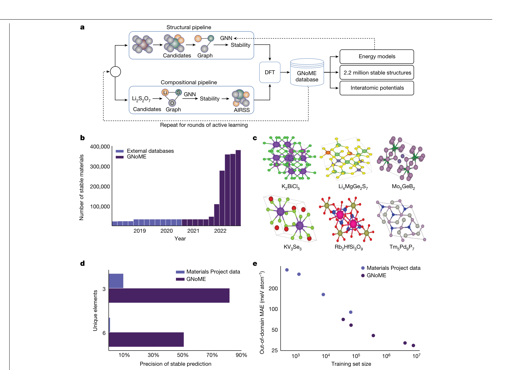
• GNoME (Merchant et al. 2023): GNN surrogates filter candidates, DFT verifies, results retrain the model — six rounds of active learning.
• 2.2 million predicted-stable crystals; 381,000 new convex-hull entries — an order-of-magnitude expansion; hit rates > 80% with structure.

• 736 of them independently made by labs worldwide — the rest are proposals.
• Step 1–2 of the loop is essentially solved at scale. Steps 3–6 — making and measuring — are the bottleneck. That is where the next slides live.

Why this slide sits here. Slide 14 said “discovery is a decision problem.” This is the strongest 2023 evidence: the prediction side scaled to millions of candidates, and the number that ended up in a vial is measured in hundreds — made by humans, incidentally, not by the loop. The asymmetry between panel (b)’s 381k hull entries and “736 experimentally matched” is the whole §E argument in two numbers.

The scaling-law point (panel e). Out-of-domain MAE falls as a power law with training data — the same shape as language-model scaling laws. This is why foundation MLIPs (supplementary deck) exist: materials ML has entered its scaling era, and the marginal cost of a prediction keeps falling while the cost of a synthesis does not.

Tie to §D. GNoME’s own validation is in-distribution DFT agreement plus r²SCAN cross-checks. Whether a specific GNoME candidate is trustworthy for your chemistry family is exactly the per-family calibration + OOD question of §D — the Leeman critique (slide 18) makes the same point from the experimental side.

16. Loop Architecture and Orchestration

Components — and the painful interfaces

• Surrogate stack + proposal layer (§A2 acquisition + §B feasibility + §D gate).
• Scheduler ↔︎ hardware: instrument SDK, vendor API, SiLA-2 / OPC-UA for cross-platform.
• Execution (synthesis hardware) and measurement (XRD, mass-spec, electrochem).
• Feedback: parser → database → retrain trigger; parsers must be schema-versioned.
• Each interface is a real engineering effort.

Use off-the-shelf glue

• Workflow engines: AiiDA (materials-native, provenance), FireWorks, Prefect / Airflow, Argo. Pick one, do not roll your own.
• BO drivers: BoTorch (modern, multi-fidelity), Ax, Dragonfly, GPyOpt. Pick one, plug it in.

The 80/20 rule for autonomous labs: 80% of the work is orchestration; 20% is the surrogate. The community has good tools for both halves now — use them.

Where the engineering hours go. A typical academic autonomous-lab build: 10% surrogate, 5% acquisition, 15% scheduler, 30% synthesis-hardware integration, 25% measurement-hardware integration, 15% parsers and databases. The ML is small; the integration is enormous.

The “do not roll your own” rule. Off-the-shelf engines handle parallelism, retry-on-failure, provenance, monitoring, resumption-from-crash. A custom engine handles none of those by default and costs a postdoc-year to make robust.

SiLA-2 / OPC-UA, one line each. SiLA-2 is the closest thing to USB-for-lab-instruments (pharma-driven); when a vendor supports it, integration takes days, otherwise months. OPC-UA is its industrial-automation cousin — heavier, real-time guarantees.

The “schema-versioned parser” point. A parser written against an instrument’s 2024 data format breaks with the 2025 firmware update. Version the schema; test against old data; have a fallback.

Why BoTorch in 2026. Multi-fidelity, batch acquisition, constrained optimisation, custom kernels — all first-class, and the plug-in architecture matches the workflow engines cleanly.

17. A-Lab — the Landmark (2023)

The A-Lab pipeline: DFT-screened air-stable targets from the Materials Project and GNoME, literature-mined synthesis recipes, robotic powder dosing → heating → XRD, ML phase identification with Rietveld confirmation, and active-learning recipe optimisation on failure. Figure: Szymanski et al., Nature 624, 86 (2023), CC BY 4.0.

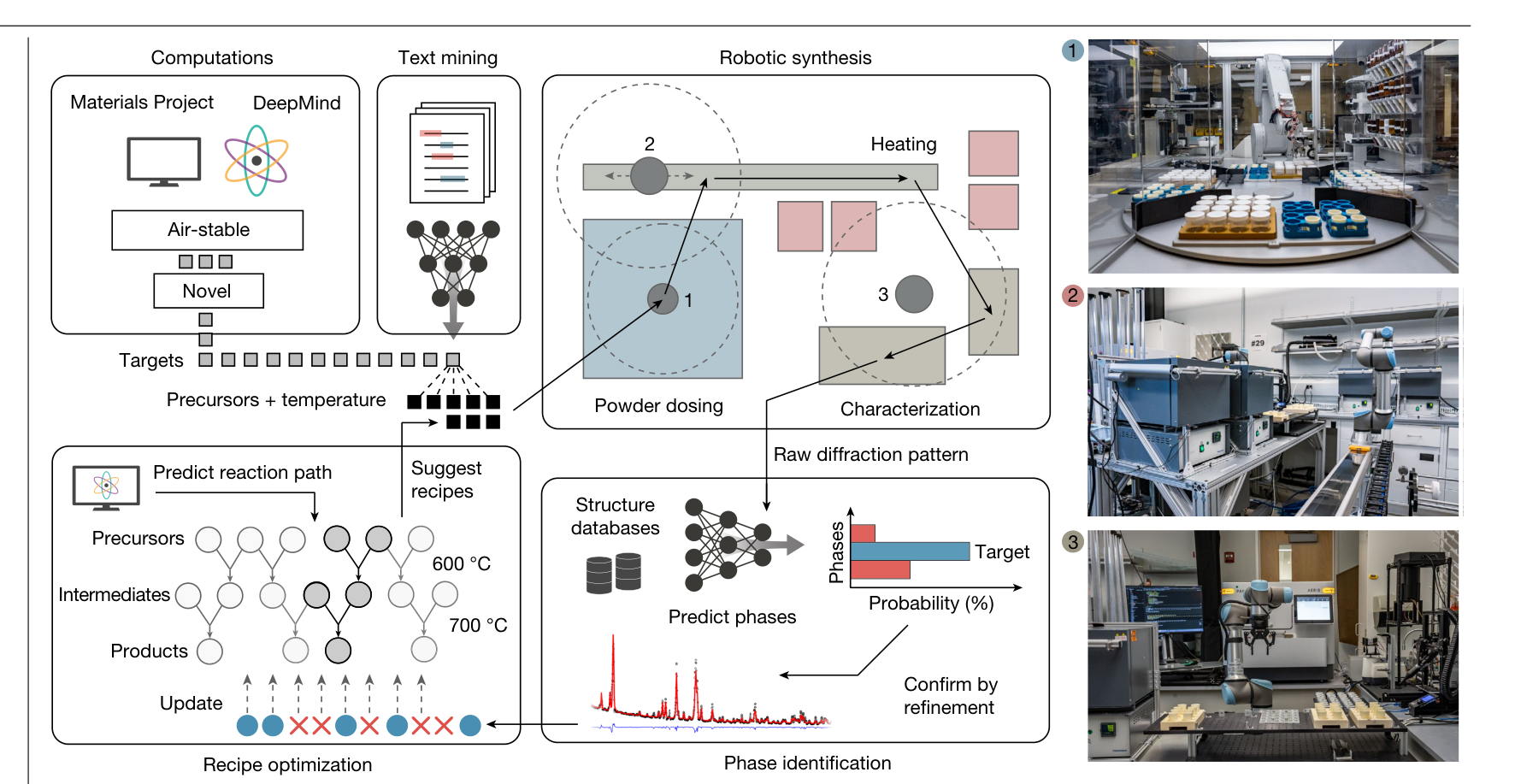
• Berkeley’s autonomous lab for inorganic powder synthesis (Szymanski et al. 2023): all six loop steps automated end-to-end — the reported campaign: 36 of 57 novel targets claimed synthesised in 17 days of continuous closed-loop operation.

Read the 2023 paper as a workflow demonstration paper, not a materials-discovery paper. The workflow is the contribution; the new materials are the by-product. Walk the figure left to right: it is literally slide 14’s six steps drawn by the people who built one — computations + text-mined recipes (steps 1–2), robotic dosing / heating / characterisation (steps 3–5), and the active-learning recipe optimiser closing the feedback edge (step 6).

Numbers to say aloud. 57 targets spanning 33 elements; 36 claimed successes in 17 days; 355 total experiments; recipes proposed by language models trained on text-mined literature syntheses, then refined by an active-learning module (ARROWS) that reasons over pairwise reactions and Materials Project driving forces. The failure analysis (slow kinetics, precursor volatility, amorphisation, DFT inaccuracy) feeds our failure-mode slide 19.

Forward link. “36 of 57” is the claimed result. The next slide is what happened when expert crystallographers re-analysed those 36 — keep the number in the room’s head.

18. The A-Lab Debate, Honestly

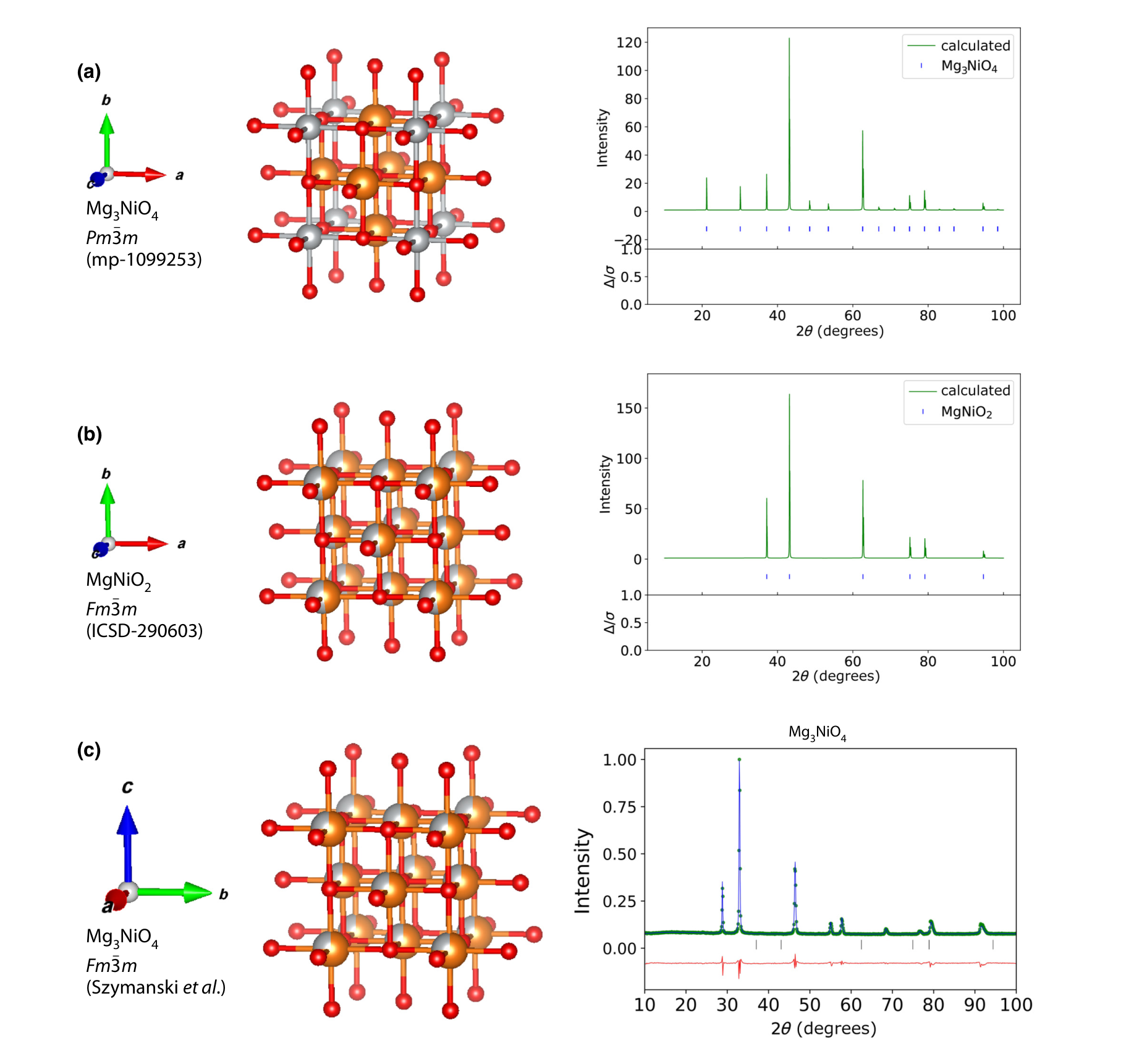
The follow-up critique (Leeman et al. 2024)

• Independent re-analysis of all claimed successes: none were demonstrably new materials.
• 24/36: predicted cation-ordered structures with no evidence for the ordering — the known compound is the same lattice with disordered cations.
• 8/36: refined against a disordered variant that already exists in the ICSD; 18/36: very poor Rietveld fits; 3/36: already reported.

• Lesson 1: autonomous synthesis works; autonomous novelty verification does not yet.
• Lesson 2: workflow result and science result need separate evaluation.
• Lesson 3: human structural review is still required for novelty claims in mid-2026 — and the field updated honestly. That is health.

The canonical example: Materials-Project-predicted cation-ordered Mg₃NiO₄ (top) vs the known disordered rocksalt MgNiO₂ (middle). The ordering would add extra superstructure reflections; A-Lab’s measured pattern (bottom) matches the disordered known compound. Figure: Leeman et al., PRX Energy 3, 011002 (2024), CC BY 4.0.

Walk the figure. Top: the prediction — Mg and Ni ordered on the cation sites, which breaks the F-centred lattice and adds superstructure peaks (e.g. the 100 reflection near 21°). Middle: the known disordered rocksalt — same aristotype, no extra peaks. Bottom: what A-Lab measured — no superstructure peaks. Occam’s razor says they made a known disordered solid solution, not the predicted new ordered compound. This is §B’s symmetry story arriving from the experimental side: the constraint the generative/screening stack ignored (disorder) is exactly where the novelty claim died.

The error taxonomy, for the exam. Four error types in the re-analysis: (1) very poor fits, 18/36; (2) refining against a different structure than predicted, 8/36; (3) predicted cation order with no evidence for it, 24/36 — the dominant one; (4) compound already reported, 3/36. Root causes: automated Rietveld refinement is not yet reliable, and compositional disorder is systematically neglected in high-throughput predictions (Materials Project and GNoME represent ordered structures only).

Where the field landed (mid-2026). Most loops now route any “novel by automated pipeline” candidate through a human structural-review queue (<5% of throughput), so the loop stays mostly automatic with a human novelty filter.

Closing rule. Every autonomous-lab paper should report two numbers: a workflow success rate, and a human-reviewed novelty rate. Neither alone is sufficient. (The broader 2023–2026 self-driving-lab landscape — Aspuru-Guzik’s ChemOS stack, polymer / electrolyte / battery loops — is in the supplementary deck; all single-domain, recipe portability unsolved.)

19. Failure Modes — Synthesis and Measurement

Synthesis side

• Recipe ambiguity: “600 °C for 12 h” — what ramp rate, crucible, atmosphere? A recipe is a full procedural object, or two platforms make two different products.
• Hardware bottleneck: weighing, mixing, thermal cycles dominate cycle time — not the surrogate.
• Sample-handling errors: dropped vials, contaminated crucibles — invisible to the model, fatal to the data. Instrument the hardware; route per-step success flags to the database.

Measurement side

• Automated phase ID returns “best match” with no warning on ambiguous patterns (slide 18); instrument calibration drifts over weeks.
• The operator-time bottleneck: 100–500 spectra / day for human review is not autonomous — it is a person staring at a screen.
• Mitigation: triage by uncertainty — auto-accept above \(\tau_{\text{high}}\), auto-reject below \(\tau_{\text{low}}\), human review between.

“An autonomous lab is a lab that fails automatically. Engineering it well means catching the failures automatically too.”

The recipe-representation point is one of the most important in materials informatics 2024–2026. Precursor identities and grades, weighing tolerance, mixing protocol, vessel material, atmosphere, ramp rate, hold time, cooling, post-treatment. The community is converging on standards (ORD for organic; inorganics still fragmented).

The cycle-time arithmetic. 30 min weighing/mixing + 6–24 h thermal cycle + 1–4 h cooling + 30 min characterisation; the surrogate takes seconds. No ML improvement helps — only parallelism and faster hardware.

War story. A polymer-electrolyte loop ran for two months before someone noticed the glovebox moisture sensor had drifted; samples were silently water-contaminated for weeks. The model “learned” that certain compositions had higher conductivity — the contaminated ones. Two months of data invalidated. Atmospheric logs are not optional.

The dirty secret. A “fully autonomous” loop in 2026 still requires 20–60% of one researcher’s time on review tasks. That is progress over the manual baseline, but it is not “autonomous.” With calibrated triage, 70–90% of cases are auto-handled and the human sees only the genuinely hard ones.

20. What Works, What Does Not — Mid-2026

Works (productive use)

• Workflow orchestration on a single platform.
• BO over single composition axes with one fast measurement endpoint.
• Synthesis-then-XRD on inorganic powders with curated phase library.
• Photochemistry with HPLC readout.
• Closed-loop within a curated chemistry family.

Marginal / does not yet work

• Multi-step synthesis with on-line correction.
• Multi-property optimisation under conflicting objectives.
• Cross-platform recipe portability.
• Open-ended novelty discovery without curated candidate pools.
• Self-debugging instruments; cross-domain transfer (catalysis ↔︎ batteries).

The honest 2026 verdict: autonomous labs are real research infrastructure, within their domain. They are not yet a general-purpose discovery engine. The minimum viable build — one platform you control end-to-end, one trusted measurement endpoint, a constrained calibrated surrogate, an off-the-shelf workflow engine, an audit trail — buys 3–5× throughput and runs nights and weekends.

Why this slide matters more than the previous five. Students will leave and read autonomous-lab marketing material; they need a calibrated frame for what to believe.

The “single composition axis” caveat. Most successful 2024–2026 loops optimised a 1D–2D composition slice with a single property target. “Vary five things at once” is research, not production, in 2026.

The “curated phase library” caveat. Inorganic loops with XRD readout work because ICSD is large and well-curated. For novel polymorphs and metastable phases the readout degrades to “we measured something; we are not sure what.”

The “open-ended novelty” caveat. Loops explore a defined search space well; they do not define it. The candidate pool comes from an MP query, a chemist, or a generative model. The loop screens; it does not invent.

Minimum viable build (full slide in the supplementary deck). One platform, one measurement, one chemistry domain succeeds in ~1 PhD-year and is the foundation to grow on — adding a second modality afterwards is days, not months. Groups that attempt the “complete” multi-domain lab first burn 2 PhD-years and fail.

§R · Module Recap — The Whole of MG in Thirty Minutes

21. The MG Syllabus Arc in One Slide

The arc, walked once more

• Physics (U2–U4): QM postulates, electronic structure, thermo, atomistic simulation.
• Representations (U6–U7): graphs, local atomic environments, descriptors.
• Models (U8–U10): regression, neural networks, learned representations.
• Geometry (U11–U12): latent spaces, clustering, discovery vs labelling.

The arc’s destination

• Decision (U13–U14): UQ, BO, constraints, trust, autonomous loops.
• Each unit served the next.
• This unit served all of them.
• The integration story is the test of whether the rest taught anything operational.

This slide launches the module recap. Walk the arc slowly here — it is the skeleton the recap will flesh out unit by unit.

The pedagogical claim made baldly. U2–U4 (physics) was the substrate for U6–U7 (representations); U6–U7 the input to U8–U10 (models); U8–U10 fed U11–U12 (geometry); U11–U12 fed the Week-13 core (§A2); §A2 fed U14. This linearity is unusual for ML courses; MG was designed to be linear, and U14 is the test of whether the linearity held.

The honest meta-comment. Some students took the course as a grab-bag; that’s fine — the arc was a scaffolding device, not a religion. But for the students who followed it, the closing-the-loop sensation matters. State it aloud.

22. U1–U2 · Quantum Mechanics: Postulates and Atoms

The core

• Classical physics broke on blackbody radiation, the photoelectric / Compton effects, and atomic spectra → energy is quantised.
• The postulates: states are wavefunctions; observables are Hermitian operators; spectral decomposition; measurement collapse; Schrödinger time evolution.
• Spin and Pauli exclusion; the variational principle — any trial wavefunction bounds the ground-state energy from above.

Why it mattered downstream

• The Hamiltonian is the object every later method approximates (U3).
• The variational principle is the engine of HF and DFT — and the ancestor of every “minimise a loss” you have run since.
• Exam angle: state a postulate precisely; apply the variational bound to a trial wavefunction.

Recap pacing. ~2.5 minutes per recap slide. Left column: what we learned. Right column: why the rest of the course needed it, plus the exam angle. Say the connective sentence out loud on every slide — the recap’s job is the arrows, not the boxes.

The one connective sentence here. “Everything in this course is an approximation to the many-electron Schrödinger equation — U1–U2 wrote it down, and the variational principle told us how to approximate it without lying about the direction of the error.”

23. U3 · Quantum Chemistry Methods (HF → DFT)

The core

• The many-electron problem is unsolvable exactly → basis sets (STOs vs GTOs; GTOs won on integral speed, fixed by contraction).
• Hartree-Fock: mean field + Slater determinant → exchange exactly, correlation missing.
• Post-HF (MP, CC) buys correlation at steep cost; DFT trades the wavefunction for the density — the workhorse.

Why it mattered downstream

• DFT is where our labels come from: formation energies, band gaps — with functional bias (PBE vs SCAN) that became §D’s sim–exp gap.
• The cost ladder (DFT hours, CC days) is why surrogates exist at all — and why slide 15’s “1000× cheaper” MLIPs changed the economics.
• Exam angle: why GTOs won; what HF misses; place DFT on the accuracy-vs-cost ladder.

The connective sentence. “Every ‘label’ in every training set of this course was produced by the methods of U3 — so every model of U8–U14 inherits U3’s biases. That is not a footnote; it is §D.”

If pressed for time. The single non-negotiable retention item is the accuracy-vs-cost ladder and DFT’s position on it.

24. U4–U5 · Thermodynamics, Statistical Mechanics, MD & MC

The core

• Free energies decide phases — which potential when (\(U, H, F, G\)); entropy and the laws.
• The partition function links micro to macro; Maxwell-Boltzmann.
• Simulation: MD integrates forces in time; Metropolis MC samples the Boltzmann distribution — detailed balance is the correctness condition.

Why it mattered downstream

• The convex hull and \(E_{\text{hull}}\) are thermodynamics — today’s acquisition target (slide 04) and A-Lab’s screening criterion.
• MD needs forces → why equivariant MLIPs (U6, U9) are non-negotiable.
• MC’s importance-sampling logic returns as Thompson sampling and BO exploration.
• Exam angle: justify the Metropolis acceptance rule; pick the right free energy for fixed \(T, p\).

The connective sentence. “Stability is not an ML concept — it is a free-energy statement. When the acquisition function ranks by expected hull improvement, it is doing U4’s thermodynamics with U13’s uncertainty.”

The \(E_{\text{hull}}\) caveat to repeat. \(E_{\text{hull}} \le 0\) at 0 K without entropy is not synthesisability — the A-Lab / Leeman story (slides 17–18) is partly this gap.

25. U6 · Descriptors and Local Atomic Environments

The core

• The descriptor ladder: composition-only (Magpie / matminer) → structure-aggregated (RDF, Voronoi coordination) → local atomic environments under a radial cutoff.
• Invariance discipline: translation, rotation, permutation, PBC — raw Cartesians are the wrong baseline.
• Local environments are the input object of universal MLIPs.

Why it mattered downstream

• Where composition-only fails = polymorphs (same formula, different structure, different property).
• §B’s architectural priors are this invariance discipline turned into network design.
• Exam angle: pick a descriptor tier for a given task and dataset size, and justify; name the four invariances.

The connective sentence. “U6 asked: what is the right coordinate system for a material? Everything after — graphs, GNNs, latent spaces — is refinement of that answer.”

The decision-tree framing to repeat. Composition-only when you have no structures and big \(n\); RDF/coordination when structures exist but locality is not resolved; local environments when you need per-atom resolution (forces, defects).

26. U7 · Crystals as Graphs

The core

• A crystal is a periodic graph: atoms as nodes, edges under a radial cutoff, PBC-aware neighbour lists (periodic images are not optional).
• Geometry becomes features via Gaussian RBF distance encoding.
• Message passing is the template every materials GNN instantiates.

Why it mattered downstream

• Invariance vs equivariance: scalar targets may be invariant; forces must be equivariant — non-negotiable.
• This representation is what the whole model stack sits on: U9’s SchNet/CGCNN, U10’s pretraining, GNoME (slide 15).
• Exam angle: sketch the graph-construction workflow; explain why equivariance is required for forces but not for energies.

The connective sentence. “U6 defined the neighbourhood; U7 made it differentiable. Message passing is ‘local environments, applied recursively’ — after \(k\) rounds, each atom has seen its \(k\)-hop chemistry.”

Common exam slip to warn about. Confusing invariance (output unchanged) with equivariance (output transforms with the input). One sentence each, then the force counter-example.

27. U8 · Regression and Generalization

The core

• Bias-variance and regularisation-as-prior (MFML W7), applied to materials descriptors.
• The “what kind of new is your test set?” taxonomy: chemistry-family leakage, polymorph aliasing, database shift, stability bias, prototype dominance.
• Split design is the experiment design: random vs group-aware vs LOCO (leave-one-chemistry-out) vs time splits.

Why it mattered downstream

• A random-split MAE headline overstates discovery performance; LOCO is the operational number — it belongs on the model card.
• U8 is why §D exists: distribution shift was already visible in the split protocol before we gave it a name.
• Exam angle: given a discovery campaign, choose and defend a split protocol; diagnose a leakage story.

The connective sentence. “U8 was the unit where materials ML stopped being MFML-with-different-data. The split protocol is a scientific claim about what ‘new’ means — and the exam will make you defend one.”

The rubric tie-in. The exam rubric’s “defensible split (LOCO or time)” line comes straight from this unit. Say so.

28. U9 · Neural Networks for Materials Properties

The core

• The MLP-on-Magpie failure: generic architectures waste capacity learning symmetries from data.
• SchNet: continuous-filter convolutions on interatomic distances. CGCNN: message passing on crystal graphs.
• Equivariant networks (NequIP, MACE): E(3) symmetry by construction → data efficiency and physical correctness.

Why it mattered downstream

• These are the step-1 surrogates of today’s loop and the backbone of foundation MLIPs — GNoME’s GNN (slide 15) is this unit at industrial scale.
• §B’s “architectural prior is the gold standard” was born here.
• Exam angle: SchNet vs CGCNN vs equivariant nets — which for molecular energies, which for crystals, which for forces, and why.

The connective sentence. “U9 is U6’s invariance discipline compiled into weights. The reason MACE needs less data than an MLP is that it does not have to learn rotational symmetry — it cannot violate it.”

The cutoff-sensitivity reminder. Smooth envelopes at the cutoff radius — small detail, recurring exam favourite, and a real failure mode in force fields.

29. U10–U11 · Representation Learning and Latent Spaces

The core

• Self-supervised pretraining on unlabelled crystal databases: atom masking, edge masking, denoising, contrastive pairs.
• Pretrained GNNs as featurizers; foundation embeddings (M3GNet, MACE).
• Latent maps of the Materials Project: colour by formation energy / band gap / \(E_{\text{hull}}\); clusters = chemistry families; the UMAP-is-not-truth pitfall.

Why it mattered downstream

• The latent space is where §D’s OOD distance is measured — “did our latent cover this candidate?” is a U10/U11 question.
• Phase discovery without labels = clustering the latent (U11).
• Exam angle: design a pretext task for a given data situation; read a property map critically (what UMAP distances do and do not mean).

The connective sentence. “U10–U11 built the map; §D used it as a fence. The nearest-neighbour OOD score on slide 12 is literally a distance in the space these units constructed.”

The pitfall to repeat. UMAP preserves neighbourhoods, not global distances — never read cluster-to-cluster distance as chemical similarity. This is a reliable exam trap.

30. U12 · Generative Models and Inverse Design

The core

• Forward vs inverse: from “predict the property of a structure” to “generate a structure with a property.”
• Diffusion on crystals: CDVAE, DiffCSP(++), MatterGen — lattice + coordinates + species, symmetry-aware variants, conditioning + DFT validation.
• Evaluation: S.U.N. — stable, unique, novel.

Why it mattered downstream

• Generative proposals are exactly what §B must constrain (Na₂Cl₃!) and §D must gate.
• The Leeman critique (slide 18) is an evaluation failure of the same kind S.U.N. tries to prevent — “novel” claimed without checking the disordered known parent.
• Exam angle: name how one named model handles symmetry / stoichiometry; critique a novelty claim with the S.U.N. vocabulary.

The connective sentence. “U12 is the proposal engine; U14 is the seatbelt. A generative model without §B’s feasibility filter and §D’s OOD gate is a Na₂Cl₃ factory with good marketing.”

The disorder blind spot, once more. Ordered-structure databases beget ordered-structure generators — the Mg₃NiO₄ story (slide 18) is what that looks like when it reaches a furnace.

31. U13 → §A2 · Uncertainty-Aware Discovery

The core (taught this morning as §A2)

• Databases and the convex hull as discovery targets; \(E_{\text{hull}}\) as the discoverability signal.
• \(\sigma\) over point predictions; the GP surrogate; EI / UCB / TS; hull-aware acquisition; the active-learning loop.

Why it mattered downstream

• The loop pentagon (slide 05) is the spine of §B, §D, §E — every section plugged into one of its edges.
• The full cancelled Week-13 deck remains optional reference on the shared drive.
• Exam angle: two candidates, same mean, different \(\sigma\) — what does each acquisition function do, and what does a trust gate add?

Keep this one fast (~90 seconds). It was taught eight slides ago; the recap job is only to place it in the arc: U13 is where prediction became decision, and U14 is where decision became defensible decision.

32. U14 · Today, in One Slide

The three knobs

• §B constraints: four families × three mechanisms; filter first, rank second; train soft, deploy hard.
• §D trust: per-family calibration + OOD score + audit trail; beware silent extrapolation.
• §E the loop: six steps; GNoME at the proposal end, A-Lab at the execution end, the debate in between; honest 2026 verdict.

The five must-know statements

1. Constraints are correctness, not regularisation.
2. Soft penalties in the loss; hard projections at acquisition; architectural priors are the gold standard.
3. Uncertainty is not coverage — calibrated only in-distribution; under shift, OOD detection + ensembles + audit trail.
4. Six loop steps; failure at any of them; audit the trail.
5. The bottleneck is synthesis and measurement, not the surrogate.

This is the promised repeat of slide 02’s five statements. Read them slowly; each is a likely exam stem.

The one-breath version of today. “We made the U13 loop honest: constraints so it cannot propose nonsense, trust gates so it cannot bluff, and an execution layer so it actually makes something — with A-Lab as proof it can run and the Leeman critique as proof it still needs a crystallographer.”

33. Rapid Self-Test — One Question per Unit

1. U2: Which postulate tells you the state after a measurement?
2. U3: Why did GTOs beat STOs despite the wrong cusp behaviour?
3. U4: Which free energy governs fixed \(T, p\) — and why is it the hull’s currency?
4. U5: What condition guarantees Metropolis samples the Boltzmann distribution?
5. U6: Name the four invariances a descriptor must respect.

6. U7: Why must force predictions be equivariant rather than invariant?
7. U8: Random-split MAE 25, LOCO 90 meV/atom — which do you report, and to whom?
8. U9: New ternary-oxide energy model: SchNet, CGCNN, or MACE — why?
9. U10–U11: Which §D OOD score lives in the latent space?
10. U12–U14: What does S.U.N. stand for — and which letter did the A-Lab critics attack?

How to run it. Cold-call or think-pair-share, ~20 seconds per question, answers oral. This slide is also the session’s time buffer: cut questions freely if running late, or linger if ahead.

Answer key. (1) Collapse postulate — post-measurement state is the eigenstate of the measured eigenvalue. (2) Gaussian product theorem → analytic integrals; contraction repairs the shape. (3) Gibbs free energy; the hull is constructed from formation free energies at fixed \(T, p\) (in practice 0 K DFT proxies). (4) Detailed balance (with ergodicity). (5) Translation, rotation, permutation, PBC. (6) Forces are vectors — they must rotate with the structure; an invariant output cannot. (7) Report both; LOCO to anyone making a discovery decision — random-split alone overstates. (8) CGCNN or MACE (crystal PBC support); MACE if forces / data efficiency matter; SchNet is molecular-first. (9) Latent-space nearest-neighbour distance (slide 12). (10) Stable, Unique, Novel — the critics attacked Novel (disordered known parents, slide 18).

Closing line before §H. “If you could answer seven of those ten, you are in good shape. The last two slides tell you exactly what the exam rewards.”

§H · Course Wrap

34. The Four Big Skills

Choose and Train

1. Choose a representation with the right invariances for the property (U6–U7, U10, §B).
2. Train a surrogate with calibrated uncertainty and a defensible split protocol (U8, §A2, §D).

Plan and Close

3. Plan an acquisition that respects feasibility, OOD coverage, and budget (§A2, §B, §D).
4. Close the loop with reviewable artefacts (audit trail, model card, run log) (§D, §E).

If you can do all four end-to-end on a chemistry domain you care about, you are an MG practitioner. That is what this course taught.

Why four and not seven. Seven would be a list of techniques; four is a list of operational competences — the answer to “what does an MG practitioner do all day?”

The exam connection. Each exam question probes one of the four skills via a scenario: “Given representation X for property Y, what invariance is needed and how do you bake it in?” “Given two acquisition strategies, which respects this constraint?” “Given a loop with this failure, what audit-trail entry is missing?”

Read aloud, slowly, for the room. “Choose. Train. Plan. Close. Four skills. Twelve units served those four. If you have those four, you have what this course taught.”

35. Exam, Questions, and End of MG

Exam scope

• The four big skills (slide 34), each via one operational scenario.
• Worked examples drawn from U8, U10, §A2, U14.
• Vocabulary: representation, invariance, kernel, posterior, calibration, OOD, feasibility, audit trail.
• Algorithms: the pseudocode side deck lists all sixteen you must be able to write and trace.

The exam rubric

• Bring to every answer: a feasibility filter, an OOD / calibration check, a defensible split (LOCO or time), a named failure mode, a mitigation.
• That is the rubric. State the constraint. State the trust signal. State the failure mode. State the mitigation.
• Thank you. Questions.

The exam framing is deliberate. MG’s exam tests integration of techniques: can you assemble the four skills on a fresh scenario? That is what practitioners actually do.

The “five things to bring to every answer” rubric. Filter + trust check + split + failure + mitigation. A student who applies these five to any prompt produces a passable answer; with detail and specificity, a strong one.

The closing line, said calmly. “Thank you. This was Materials Genomics. The course tried to prepare you to do four things end-to-end. If it succeeded, you are ready to start a master’s thesis or a PhD in this area. The reading list is in the supplementary deck. Questions?”

Bishop, Christopher M. 2006. Pattern Recognition and Machine Learning. Springer.

Goodfellow, Ian, Yoshua Bengio, and Aaron Courville. 2016. Deep Learning. MIT Press.

Leeman, Josh, Yuhan Liu, Joseph W. Stiles, et al. 2024. “Challenges in High-Throughput Inorganic Materials Prediction and Autonomous Synthesis.” PRX Energy 3 (1): 011002. https://doi.org/10.1103/prxenergy.3.011002.

Merchant, Amil, Simon Batzner, Samuel S. Schoenholz, Muratahan Aykol, Gowoon Cheon, and Ekin Dogus Cubuk. 2023. “Scaling Deep Learning for Materials Discovery.” Nature 624 (7990): 80–85. https://doi.org/10.1038/s41586-023-06735-9.

Neuer, Michael et al. 2024. Machine Learning for Engineers: Introduction to Physics-Informed, Explainable Learning Methods for AI in Engineering Applications. Springer Nature.

Sandfeld, Stefan et al. 2024. Materials Data Science. Springer.

Szymanski, Nathan J., Bernardus Rendy, Yuxing Fei, et al. 2023. “An Autonomous Laboratory for the Accelerated Synthesis of Inorganic Materials.” Nature 624 (7990): 86–91. https://doi.org/10.1038/s41586-023-06734-w.

Continue

• ← Previous: Unit 13 — Uncertainty-Aware Discovery & Gaussian Processes (optional reference — lecture cancelled, core folded into Unit 14)
• All courses