Mathematical Foundations of AI & ML
Unit 9: Representation Learning
Prof. Dr. Philipp Pelz
FAU Erlangen-Nürnberg
Title + Unit 9 positioning
- Unit 8 introduced probabilistic foundations. Unit 9 asks: what should the model actually see?
- The quality of the input representation determines the ceiling for any learning algorithm.
- Representation learning: letting the model discover useful features from raw data.
Learning outcomes for Unit 9
By the end of this lecture, students can:
- explain the manifold hypothesis and why high-dimensional data admits low-dimensional representations,
- contrast handcrafted features with learned representations,
- derive the autoencoder objective and relate it to PCA,
- apply autoencoders to compression, anomaly detection, and feature extraction.
Why features matter more than algorithms
- A good representation makes a simple model effective; a bad one makes even complex models fail.
- Traditional ML pipeline: raw data \(\to\) feature engineering \(\to\) model \(\to\) prediction.
- Deep learning promise: raw data \(\to\) learned representation \(\to\) prediction — end-to-end.
The curse of dimensionality
- In high-dimensional spaces, data points become equidistant — distances lose meaning.
- To cover a \(d\)-dimensional space uniformly, sample size must grow exponentially with \(d\).
- Practical consequence: models need far more data in high dimensions, or we must reduce dimensionality.
The manifold hypothesis
- Key idea: real-world data does not fill the full ambient space \(\mathbb{R}^d\).
- Instead, data concentrates on or near a low-dimensional manifold embedded in \(\mathbb{R}^d\).
- Example: images of faces form a tiny subspace of all possible pixel arrays.
- Dimensionality reduction = finding this manifold.
Visual: Swiss roll and manifold structure
- The Swiss roll: 3D data that actually lives on a 2D surface.
- Linear methods (PCA) project onto a plane — they cannot “unroll” the manifold.
- Nonlinear methods can recover the intrinsic 2D structure.
- This illustrates why we need methods beyond PCA.
PCA recap (Unit 2)
- PCA finds the linear subspace that captures maximum variance:
- Compute covariance matrix \(\mathbf{\Sigma}\).
- Eigendecomposition: \(\mathbf{\Sigma} = \mathbf{V} \mathbf{\Lambda} \mathbf{V}^\top\).
- Project onto top-\(k\) eigenvectors.
- Optimal linear dimensionality reduction under MSE [@bishop2006pattern].
Limitations of PCA
- PCA can only find flat subspaces (hyperplanes through the origin).
- It fails when the data manifold is curved, folded, or has nonlinear structure.
- PCA also struggles with multi-modal data — it finds one global direction, not local structure.
- We need nonlinear alternatives.
Handcrafted features — historical approach
- Before deep learning, domain experts designed features manually:
- Spectroscopy: peak positions, widths, areas.
- Materials: grain size distribution, composition ratios.
- Images: SIFT descriptors, Gabor filters.
- This requires deep domain knowledge and is labor-intensive.
Handcrafted vs learned features
Handcrafted Features
- Design effort: High (expert required)
- Interpretability: High (physical parameters)
- Flexibility: Brittle to new domains
- Data requirements: Low
- Best when: Domain knowledge is strong
Learned Features
- Design effort: Low (fully data-driven)
- Interpretability: Lower (latent representations)
- Flexibility: Highly adaptive to data
- Data requirements: High
- Best when: Data is abundant
| Aspect | Handcrafted | Learned |
|---|---|---|
| Design effort | High | Low |
| Interpretability | High | Lower |
| Flexibility | Brittle | Adaptive |
| Data requirements | Low | High |
| Best when | Domain knowledge | Data is abundant |
The autoencoder idea
- Train a neural network to reconstruct its own input: \(\hat{\mathbf{x}} = g(f(\mathbf{x}))\).
- The catch: force the data through a bottleneck (low-dimensional latent layer).
- The network must learn to compress the essential information and discard the rest [@neuer2024machine].
Encoder-decoder architecture
- Encoder \(f_\phi\): maps input to latent code: \(\mathbf{z} = f_\phi(\mathbf{x})\), where \(\mathbf{z} \in \mathbb{R}^{d_z}\).
- Decoder \(g_\psi\): maps latent code back to input space: \(\hat{\mathbf{x}} = g_\psi(\mathbf{z})\).
- The encoder discovers the representation; the decoder ensures it is sufficient.
The bottleneck constraint
- Input dimension \(d_x \gg\) latent dimension \(d_z\).
- The bottleneck forces the network to learn a compressed representation.
- If \(d_z = d_x\), the network can learn the trivial identity — no compression, no useful features.
- Choosing \(d_z\) controls the information-compression tradeoff.
Autoencoder loss function
\[ \mathcal{L} = \frac{1}{N}\sum_{i=1}^{N} \|\mathbf{x}_i - g_\psi(f_\phi(\mathbf{x}_i))\|^2 \]
- Minimize the reconstruction error across the training set.
- The network learns to preserve the most important information through the bottleneck.
- MSE is the standard choice; other losses (e.g., binary cross-entropy for pixel data) are also used.
Hourglass topology
- Input layer (wide) \(\to\) encoder layers (narrowing) \(\to\) bottleneck (narrow) \(\to\) decoder layers (widening) \(\to\) output layer (wide).
- The symmetric shape gives the architecture its name.
- Layer widths typically decrease/increase by factors of 2 [@mcclarren2021machine].
Linear autoencoder = PCA
- Theorem: a linear autoencoder with MSE loss learns the same subspace as the top-\(k\) PCA components.
- The encoder weights span the principal subspace; the decoder performs the reconstruction.
- This makes the autoencoder a strict generalization of PCA.
- Adding nonlinear activations is what makes autoencoders more powerful.
Why nonlinearity matters
- Nonlinear activations (ReLU, sigmoid) allow the autoencoder to learn curved mappings.
- A nonlinear autoencoder can capture manifold structure that PCA misses.
- Example: on the Swiss roll, a 2-unit bottleneck autoencoder with ReLU recovers the 2D coordinates; PCA cannot.
Choosing the bottleneck dimension
- Too large (\(d_z \approx d_x\)): no compression, trivial identity, no useful features.
- Too small (\(d_z = 1\) for complex data): lossy compression, important structure lost.
- Just right: captures the intrinsic dimensionality of the data manifold.
- Practical approach: sweep \(d_z\) and plot reconstruction error vs latent dimension.
Reconstruction error vs latent dimension
- Plot RMSE vs \(d_z\): typically a sharp elbow where adding more dimensions yields diminishing returns.
- The elbow indicates the intrinsic dimensionality of the data.
- Compare to PCA with the same number of components — the AE curve is typically lower for curved manifolds.
Training an autoencoder
- Same training procedure as any neural network:
- Forward pass: encode \(\to\) latent \(\to\) decode.
- Compute reconstruction loss.
- Backward pass: compute gradients via backpropagation.
- Update weights via optimizer (Adam, SGD).
- Standard practices apply: mini-batches, learning rate schedules, early stopping.
Regularization in autoencoders
- Without regularization, autoencoders can memorize training samples.
- Weight decay: prevents large weights.
- Dropout: prevents co-adaptation of encoder features.
- Noise injection: denoising autoencoder (see slides 28-30).
- Regularization ensures the latent code captures generalizable structure.
Checkpoint: autoencoder vs PCA
- Question: When does a nonlinear autoencoder outperform PCA?
- Answer: When the data manifold is curved or has nonlinear structure.
- For data on a flat subspace, PCA and a linear AE are equivalent.
- The advantage of autoencoders grows with manifold complexity.
Convolutional autoencoders — motivation
- For image, spectral, or spatial data, fully connected layers ignore spatial structure.
- Convolutional layers exploit local patterns and translation equivariance.
- A convolutional autoencoder preserves spatial relationships in the latent representation [@mcclarren2021machine].
Encoder: strided convolutions
- A convolution with stride \(s > 1\) simultaneously:
- Extracts local features (via the learned kernel).
- Reduces spatial resolution by factor \(s\).
- No separate pooling layer needed — the downsampling is learnable.
Decoder: transposed convolutions
- Transposed (fractionally strided) convolutions perform learned upsampling.
- They reverse the spatial compression of the encoder.
- Each transposed conv layer increases spatial resolution by its stride factor.
- Alternative: nearest-neighbor upsampling + regular convolution (avoids checkerboard artifacts).
Convolutional autoencoder architecture
- Encoder: Input \(\to\) Conv(stride=2) \(\to\) ReLU \(\to\) Conv(stride=2) \(\to\) ReLU \(\to\) Flatten \(\to\) Dense \(\to\) \(\mathbf{z}\).
- Decoder: \(\mathbf{z}\) \(\to\) Dense \(\to\) Reshape \(\to\) TransConv(stride=2) \(\to\) ReLU \(\to\) TransConv(stride=2) \(\to\) Output.
- Symmetric encoder-decoder structure with matching layer dimensions.
Pooling vs strided convolutions
- Max/avg pooling: fixed operation, discards spatial information, not learnable.
- Strided convolutions: learnable downsampling, jointly optimized with the rest of the network.
- Modern architectures increasingly prefer strided convolutions over pooling.
- For the decoder, transposed convolutions reverse the strided convolutions.
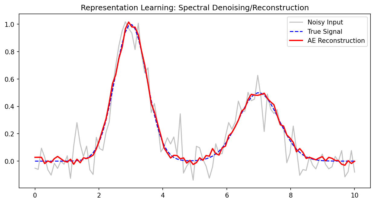
Denoising autoencoders
- Standard AE: input = target = \(\mathbf{x}\).
- Denoising AE: input = corrupted \(\tilde{\mathbf{x}} = \mathbf{x} + \epsilon\), target = clean \(\mathbf{x}\).
\[ \mathcal{L} = \frac{1}{N}\sum_{i=1}^{N} \|\mathbf{x}_i - g_\psi(f_\phi(\tilde{\mathbf{x}}_i))\|^2 \]
- The network must learn to separate signal from noise [@neuer2024machine].
Why denoising helps
- Forces the encoder to learn robust features that capture the underlying structure, not noise.
- The latent code must represent the clean signal — noisy details are discarded.
- Denoising AEs produce smoother, more generalizable latent representations.
Denoising autoencoder as regularization
- Adding input noise is a form of data augmentation and implicit regularization.
- It prevents the AE from learning the trivial identity mapping.
- Even when the bottleneck is relatively wide, denoising prevents memorization.
- The noise level is a hyperparameter controlling the regularization strength.
Sparse autoencoders (brief)
- Add a sparsity penalty on the latent activations:
\[ \mathcal{L} = \mathcal{L}_{rec} + \beta \sum_j \text{KL}(\rho \| \hat{\rho}_j) \]
- Encourages most latent units to be inactive for any given input.
- Result: each input activates only a few latent features — interpretable, disentangled.
- Useful when the bottleneck is wide but we want selective feature activation.
Checkpoint: convolutional AE design
- Problem: You have 128×128 spectral images. Design an encoder with three strided conv layers.
- Layer 1: 128×128 → 64×64 (stride=2, 32 filters).
- Layer 2: 64×64 → 32×32 (stride=2, 64 filters).
- Layer 3: 32×32 → 16×16 (stride=2, 128 filters).
- Flatten + Dense → 16-dim latent code. Compression: 16384 → 16.
Application 1: data compression
- Store the latent code \(\mathbf{z}\) instead of the full input \(\mathbf{x}\).
- Decode on demand when the original data is needed.
- Compression ratio: \(r = d_x / d_z\). Example: 2000-dim spectrum → 10-dim code = 200× compression.
- Quality measured by reconstruction RMSE or structural similarity.
Compression ratio and reconstruction quality
- Higher compression (smaller \(d_z\)): more information lost, higher reconstruction error.
- The optimal tradeoff depends on the application:
- Archival storage: accept some loss for high compression.
- Real-time reconstruction: minimize latency and error.
- Always evaluate on held-out data to ensure generalization.
Application 2: anomaly detection via reconstruction error
- Train the AE on normal data only.
- At test time, compute reconstruction error for each sample.
- Normal samples: low error (the AE has learned to reconstruct them).
- Anomalous samples: high error (they differ from the learned patterns) [@neuer2024machine].
Setting the anomaly threshold
- Compute the reconstruction error distribution on validation normal samples.
- Set threshold at the 95th or 99th percentile — depending on tolerance for false alarms.
- Samples exceeding the threshold are flagged as anomalies.
- The threshold can be tuned based on the cost of false positives vs false negatives.
Application 2b: anomaly detection via latent space outliers
- Normal data forms clusters in the latent space.
- Anomalies map to regions far from these clusters.
- Detection: compute distance to nearest cluster centroid or use density estimation in latent space.
- This catches structurally novel anomalies even if reconstruction error is moderate.
Two anomaly strategies compared
| Strategy | Catches | Misses |
|---|---|---|
| Reconstruction error | Any deviation from normal | Anomalies that happen to reconstruct well |
| Latent outlier | Structural novelty | Anomalies close to normal manifold |
- Best practice: use both strategies together for robust anomaly detection.
Application 3: feature extraction for downstream tasks
- Train an autoencoder on a large unlabeled dataset (unsupervised).
- Discard the decoder; use the encoder’s latent code as features.
- Train a simple supervised model (linear classifier, small MLP) on top of these features.
- The autoencoder extracts useful features without requiring labels.
Transfer learning with autoencoders
- Pretrain the autoencoder on a large unlabeled dataset (e.g., all available spectra).
- Fine-tune the encoder with a small labeled dataset for a specific task.
- The pretrained encoder provides a strong initialization — reduces data requirements for the supervised task.
- This is especially valuable when labels are expensive (e.g., destructive testing).
Stacking autoencoders
- Train multiple autoencoders in sequence:
- AE1: \(\mathbf{x} \to \mathbf{z}_1\) (raw → first-level features).
- AE2: \(\mathbf{z}_1 \to \mathbf{z}_2\) (first → second-level features).
- Each level captures increasingly abstract representations.
- Historical significance: this was one of the first approaches to training deep networks [@neuer2024machine].
Checkpoint: anomaly detection design
- Scenario: Your autoencoder reconstructs all training samples with RMSE < 0.05. A new sample has RMSE = 0.15 — three times the maximum training error.
- Question: Is it anomalous?
- Answer: Very likely yes. The reconstruction error is far outside the normal range, indicating the input differs significantly from learned patterns.
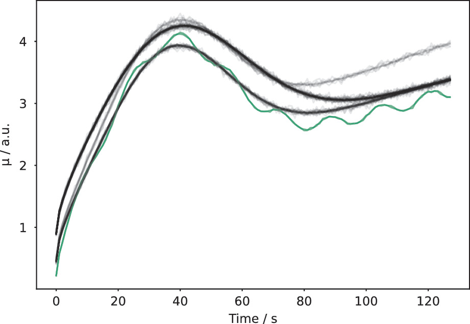
Case study: leaf spectra compression
- Near-infrared spectra with 2000 wavelength channels per sample.
- Autoencoder compresses to 10-dim latent code with < 2% reconstruction error.
- PCA with 10 components achieves ~5% error — the AE captures nonlinear spectral relationships [@mcclarren2021machine].
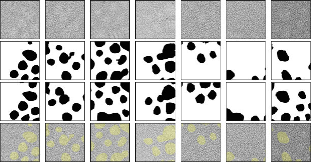
Case study: physics simulation data reduction
- Finite element simulations produce large temperature/stress field outputs (e.g., 256×256 per time step).
- A convolutional AE compresses each field to ~20 latent values.
- Enables fast storage, retrieval, and surrogate modeling from the compressed representations.
Case study: industrial anomaly detection
- Manufacturing sensor data: vibration, temperature, pressure recorded continuously.
- AE trained on 6 months of normal operation data.
- Reconstruction error spikes correlate with equipment faults detected 2-4 hours before traditional alarms.
- Provides early warning capability for predictive maintenance.
Uncertainty in autoencoder outputs
- Reconstruction error as uncertainty proxy: high error indicates the input is far from the training distribution.
- Regions of high reconstruction error correspond to regions of high epistemic uncertainty.
- This connects to Unit 8: the autoencoder implicitly flags extrapolation [@neuer2024machine].
Lecture-essential vs exercise content split
- Lecture: manifold hypothesis, AE formalism, PCA connection, convolutional/denoising variants, application design.
- Exercise: build AE in PyTorch, bottleneck dimension sweep, PCA comparison, anomaly detection, denoising demo.
Exercise setup: autoencoder for 1D signals
- Build a fully connected AE for synthetic Gaussian pulses (varying width, position).
- Train on normal cases; visualize the 2D latent space.
- Sweep bottleneck dimension and compare reconstruction error to PCA.
- Inject anomalous signals and detect via reconstruction error and latent outlier methods.
Exam-aligned summary: 10 must-know statements
- The manifold hypothesis: real data lives on a low-dimensional manifold in high-dimensional space.
- An autoencoder learns compressed representations by reconstructing input through a bottleneck.
- A linear autoencoder with MSE loss is equivalent to PCA.
- Nonlinear autoencoders capture curved manifolds that PCA cannot.
- The bottleneck dimension controls the compression-quality tradeoff.
- Strided convolutions perform learnable downsampling; transposed convolutions perform upsampling.
- Denoising autoencoders learn robust features by reconstructing clean targets from noisy inputs.
- Anomaly detection: high reconstruction error or latent outlier status flags anomalies.
- Autoencoder latent codes serve as learned features for downstream supervised tasks.
- Reconstruction error provides an uncertainty proxy for autoencoder predictions.
References + reading assignment for next unit
- Required reading before Unit 10:
- Neuer: Ch. 5.5
- McClarren: Ch. 8
- Optional depth:
- Murphy: Ch. 12 (latent linear models)
- Bishop: Ch. 12 (probabilistic PCA)
- Next unit: Latent Spaces and Embeddings — variational autoencoders, structured latent spaces, and generative models.