Mathematical Foundations of AI & ML
Unit 10: Latent Spaces and Embeddings

Prof. Dr. Philipp Pelz

FAU Erlangen-Nürnberg

Title + Unit 10 positioning

• Unit 9 introduced autoencoders as representation learners.
• Unit 10 dives deeper: what is the structure of the latent space, and how do we visualize and exploit it?
• We also introduce t-SNE, UMAP, and kernel PCA for nonlinear dimensionality reduction.

Learning outcomes for Unit 10

By the end of this lecture, students can:

• define latent spaces formally and distinguish them from raw feature spaces,
• derive the t-SNE objective and explain the crowding problem,
• compare t-SNE, UMAP, and kernel PCA for visualization and dimensionality reduction,
• use latent-space distributions for anomaly detection and trust assessment.

What is a latent space?

• A latent space is a low-dimensional space that captures the essential variation of high-dimensional data.
• “Latent” = hidden — these variables are not directly observed but inferred from the data.
• Every dimensionality reduction method (PCA, autoencoders, t-SNE) defines a latent space.

Latent space vs feature space vs PCA eigenspace

Space	Definition	Structure
Feature space	Raw measurements (\(\mathbb{R}^d\))	High-dimensional, redundant
PCA eigenspace	Linear projection onto top eigenvectors	Flat subspace, orthogonal axes
Latent space	Learned embedding (possibly nonlinear)	Captures manifold structure

Why latent spaces matter

• Compression: store data efficiently as latent codes.
• Visualization: project to 2D/3D for exploration.
• Generation: sample from latent space to create new data.
• Anomaly detection: identify out-of-distribution points.
• Downstream prediction: use latent features as inputs to supervised models.

Recap: autoencoder as latent space constructor

• Encoder \(f_\phi: \mathbb{R}^{d_{\mathbf{x}}} \to \mathbb{R}^{d_{\mathbf{z}}}\) maps each input to a latent code.
• The collection \(\{\mathbf{z}_i = f_\phi(\mathbf{x}_i)\}\) forms a point cloud in the latent space.
• The decoder \(g_\psi\) ensures the latent code retains enough information for reconstruction.

graph LR
    A[Input Data x] --> B[Encoder f_phi]
    B --> C((Latent Space z))
    C --> D[Decoder g_psi]
    D --> E[Reconstruction x']
    style C fill:#f9f,stroke:#333,stroke-width:4px

Embeddings: points in latent space

• An embedding assigns each data point a coordinate in the latent space.
• Good embeddings preserve meaningful relationships:
  • Similar inputs \(\to\) nearby embeddings.
  • Different inputs \(\to\) distant embeddings.
• The quality of the embedding determines the utility of the latent space.

What makes a good latent space?

• Neighborhood preservation: similar data points remain neighbors.
• Smoothness: small changes in latent coordinates produce small changes in decoded output.
• Continuity: no “holes” — every point in the latent space decodes to something meaningful.
• Disentanglement (ideal): each latent dimension corresponds to one interpretable factor of variation.

Latent space geometry: clusters and manifolds

• Clusters: discrete categories form separated groups in latent space.
• Manifolds: continuous variation creates smooth surfaces or curves.
• Mixed: clusters connected by low-density paths — partially continuous, partially discrete.
• The geometry reflects the structure of the data [@neuer2024machine].

Roadmap of today’s 90 min

• 10–25 min: Autoencoder latent space structure and interpretation.
• 25–40 min: Latent space geometry, interpolation, arithmetic.
• 40–55 min: t-SNE — derivation and application.
• 55–65 min: UMAP and kernel PCA.
• 65–80 min: Anomaly detection and trust quantification in latent space.

Autoencoder latent neurons: what do they encode?

• Each latent dimension captures a learned factor of variation.
• Example (spectral data): one latent neuron encodes peak position, another encodes peak width.
• These factors are discovered automatically — no human labeling required.
• But: factors may be entangled (mixed together) in standard autoencoders [@neuer2024machine].

Visualizing 2D latent spaces

• When \(d_{\mathbf{z}} = 2\), the latent space can be plotted directly.
• Color points by class label or continuous property to reveal structure.
• Well-separated colored clusters indicate the AE has learned discriminative features.
• Overlapping colors indicate ambiguity or insufficient bottleneck capacity.

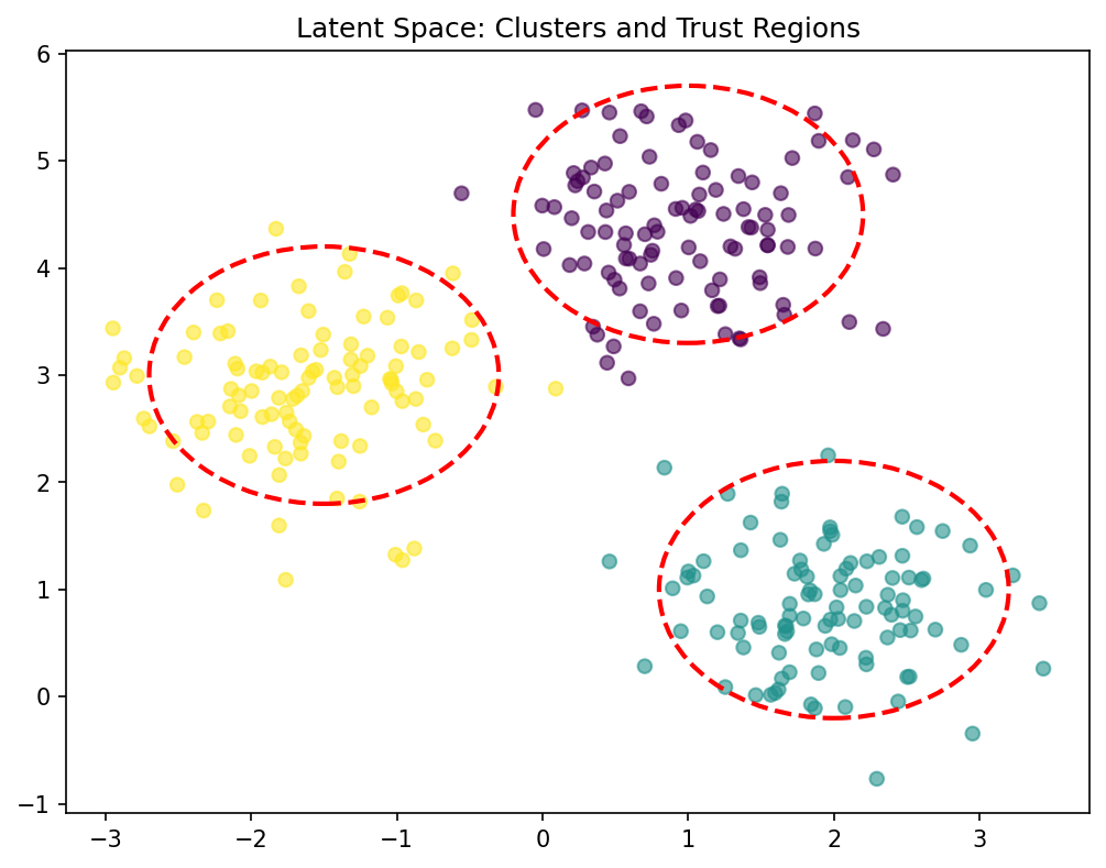
Interpreting latent space clusters

• Tight, separated clusters: distinct data modes that the AE can distinguish.
• Overlapping clusters: similar classes or insufficient latent capacity.
• Elongated clusters: continuous variation within a class (e.g., material composition gradient).
• Cluster structure informs downstream tasks: classification boundaries follow cluster separations.

Latent space interpolation

• Linearly interpolate between two latent codes: \(\mathbf{z}_{\text{mix}} = \alpha \mathbf{z}_1 + (1-\alpha) \mathbf{z}_2\)
• Decode \(\mathbf{z}_{\text{mix}}\) to observe structural transitions.
• Example: Latent space encodes [frequency, phase]. Interpolating yields smooth structural changes in the generated waveform.
• Smooth interpolation proves the latent space has learned a meaningful, continuous representation.

//| echo: false
viewof alpha_interp = Inputs.range([0, 1], {value: 0.5, step: 0.01, label: "α (Interpolation)"})

z1_latent = [1, 0]      // freq 1, phase 0
z2_latent = [5, Math.PI] // freq 5, phase pi

z_mix_latent = [
  alpha_interp * z1_latent[0] + (1 - alpha_interp) * z2_latent[0],
  alpha_interp * z1_latent[1] + (1 - alpha_interp) * z2_latent[1]
]

x_interp = d3.range(0, 4 * Math.PI, 0.05)

Plot.plot({
  width: 550,
  height: 350,
  y: {domain: [-1.2, 1.2], label: "Decoded Output"},
  x: {domain: [0, 4 * Math.PI], label: "x"},
  marks: [
    Plot.ruleY([0]),
    Plot.line(x_interp, {x: d => d, y: d => Math.sin(z1_latent[0] * d + z1_latent[1]), stroke: "black", strokeOpacity: 0.2}),
    Plot.line(x_interp, {x: d => d, y: d => Math.sin(z2_latent[0] * d + z2_latent[1]), stroke: "black", strokeOpacity: 0.2}),
    Plot.line(x_interp, {x: d => d, y: d => Math.sin(z_mix_latent[0] * d + z_mix_latent[1]), stroke: "blue", strokeWidth: 3, title: "Interpolated"}),
    Plot.text([[2 * Math.PI, 1.1]], {text: [`Freq: ${z_mix_latent[0].toFixed(2)}, Phase: ${(z_mix_latent[1]/Math.PI).toFixed(2)}π`], fill: "blue", fontSize: 16})
  ]
})

Latent space arithmetic

• Compute “concept vectors” by averaging latent codes of a category.
• Perform arithmetic: \(\mathbf{z}_{\text{result}} = \mathbf{z}_A + (\bar{\mathbf{z}}_B - \bar{\mathbf{z}}_C)\).
• Famous example (word embeddings): king − man + woman ≈ queen.
• This works when the latent space disentangles the relevant factors.

The issue of latent space structure

• Standard autoencoders produce unstructured latent spaces.
• There may be “holes” — regions where no training data maps — and decoding produces nonsense.
• The latent space is not designed for sampling or generation.
• This motivates variational autoencoders (VAEs), covered in a later unit.

Preview: variational autoencoders (VAEs)

• VAEs impose a prior (typically Gaussian) on the latent space.
• The encoder outputs a distribution \(q(\mathbf{z}|\mathbf{x})\), not a point.
• The loss includes a KL-divergence term that regularizes the latent space.
• Result: a continuous, smooth latent space suitable for generation.

Checkpoint: latent space quality

• Question: Your 2D latent space has a large empty region between two clusters. What does this mean?
• Answer: The AE has not seen data in that region — decoding points from the gap may produce artifacts. This indicates a discontinuous latent space (typical for standard AEs, addressed by VAEs).

t-SNE: purpose and overview

• t-Distributed Stochastic Neighbor Embedding (van der Maaten & Hinton, 2008).
• Purpose: visualization of high-dimensional data in 2D or 3D.
• Key idea: preserve local neighborhood structure while allowing global distortion.
• Not for feature extraction or downstream ML — purely for visualization [@mcclarren2021machine].

Step 1: Gaussian similarities in high dimensions

• For each pair \((i, j)\), define the conditional probability that \(j\) is a neighbor of \(i\):

\[ p_{j|i} = \frac{\exp(-\|\mathbf{x}_i - \mathbf{x}_j\|^2 / 2\sigma_i^2)}{\sum_{k \neq i}\exp(-\|\mathbf{x}_i - \mathbf{x}_k\|^2 / 2\sigma_i^2)} \]

• \(\sigma_i\) is chosen per point to achieve a target perplexity.

Perplexity parameter

• Perplexity \(\approx\) effective number of neighbors considered for a point.
  • Low (e.g. 5): local structure, many clusters.
  • High (e.g. 50): broader neighborhoods.
• The algorithm adjusts \(\sigma_i\) to match the target perplexity. Dense regions get smaller \(\sigma_i\), sparse get larger.
• Adjust \(\sigma_i\) to see how the neighborhood probability \(p_{j|i}\) changes for the red point.

//| echo: false
viewof sigma_tsne = Inputs.range([0.1, 4], {value: 1, step: 0.1, label: "Bandwidth (σ_i)"})

pts_tsne = [-3, -2, -0.5, 0, 0.8, 2.5, 4]
target_idx_tsne = 3

function p_ji_tsne(idx_i, idx_j, sigma) {
  if (idx_i === idx_j) return 0;
  let dist_sq = (pts_tsne[idx_i] - pts_tsne[idx_j])**2;
  let num = Math.exp(-dist_sq / (2 * sigma * sigma));
  let den = 0;
  for (let k = 0; k < pts_tsne.length; k++) {
    if (k !== idx_i) {
      den += Math.exp(-((pts_tsne[idx_i] - pts_tsne[k])**2) / (2 * sigma * sigma));
    }
  }
  return num / den;
}

tsne_data = pts_tsne.map((x, i) => ({
  x: x,
  p: p_ji_tsne(target_idx_tsne, i, sigma_tsne),
  is_target: i === target_idx_tsne
}))

Plot.plot({
  width: 550,
  height: 350,
  x: {domain: [-4.5, 4.5], label: "Data points (1D Space)"},
  y: {domain: [-0.1, 1], label: "Probability p_{j|i}"},
  marks: [
    Plot.ruleY([0]),
    Plot.line(d3.range(-5, 5, 0.1), {
      x: d => d, 
      y: d => Math.exp(-Math.pow(d - pts_tsne[target_idx_tsne], 2) / (2 * sigma_tsne * sigma_tsne)), 
      stroke: "gray", strokeDasharray: "4"
    }),
    Plot.ruleX(tsne_data.filter(d => !d.is_target), {x: "x", y1: 0, y2: "p", stroke: "blue", strokeWidth: 4}),
    Plot.dot(tsne_data.filter(d => !d.is_target), {x: "x", y: "p", fill: "blue", r: 6}),
    Plot.dot(tsne_data, {x: "x", y: -0.02, fill: d => d.is_target ? "red" : "black", r: d => d.is_target ? 8 : 5})
  ]
})

Step 2: Student-t similarities in low dimensions

• In the 2D embedding space, similarities are defined using a Student-t distribution (1 degree of freedom):

\[ q_{ij} = \frac{(1 + \|\mathbf{y}_i - \mathbf{y}_j\|^2)^{-1}}{\sum_{k \neq l}(1 + \|\mathbf{y}_k - \mathbf{y}_l\|^2)^{-1}} \]

• The heavy tails of the Student-t distribution allow distant points to spread out in the embedding, avoiding the crowding problem.

The crowding problem: why heavy tails?

• In high dimensions, the available volume grows exponentially. Many points can be mutually almost equidistant.
• When mapped to 2D, they naturally crowd into a small area.
• Using a Gaussian in both spaces \(\to\) points collapse together.
• Student-t has heavier tails: to achieve the same similarity \(q_{ij}\) for moderately similar points, they must be placed further apart in 2D space.

//| echo: false
viewof distScale = Inputs.range([1, 10], {value: 4, step: 0.1, label: "Viewing Distance"})

x_vals_t = d3.range(-distScale, distScale, distScale/200)

Plot.plot({
  width: 550,
  height: 350,
  y: {domain: [0, 0.45], label: "Similarity / Density"},
  x: {domain: [-distScale, distScale], label: "Distance ||y_i - y_j||"},
  marks: [
    Plot.ruleY([0]),
    Plot.line(x_vals_t, {x: d => d, y: d => Math.exp(-d*d/2) / Math.sqrt(2*Math.PI), stroke: "blue", strokeWidth: 3}),
    Plot.line(x_vals_t, {x: d => d, y: d => Math.PI**(-1) * (1 + d*d)**(-1), stroke: "red", strokeWidth: 3}),
    Plot.text([[distScale*0.5, 0.4]], {text: ["Gaussian similarity"], fill: "blue", fontSize: 16}),
    Plot.text([[distScale*0.5, 0.35]], {text: ["Student-t similarity"], fill: "red", fontSize: 16})
  ]
})

Step 3: KL divergence minimization

• Minimize the KL divergence between high-dim (\(\mathbf{P}\)) and low-dim (\(\mathbf{Q}\)) similarities:

\[ \text{KL}(\mathbf{P} \| \mathbf{Q}) = \sum_{i \neq j} p_{ij} \log \frac{p_{ij}}{q_{ij}} \]

• Optimize the embedding coordinates \(\{\mathbf{y}_i\}\) via gradient descent.

• Asymmetric KL: heavily penalizes nearby points being mapped far apart.

t-SNE: what it preserves

• Preserves: local neighborhood structure (nearby points stay nearby).
• Does NOT preserve: global distances, cluster sizes, cluster positions.
• t-SNE is a nonparametric method — it computes embeddings for fixed data, not a mapping function.
• New data points cannot be projected without rerunning the entire algorithm.

t-SNE: common misinterpretations

• Cluster size is meaningless: tight clusters are not “tighter” in the original space.
• Inter-cluster distance is meaningless: far-apart clusters are not necessarily far apart originally.
• Topology can change with hyperparameters: different perplexity values produce different layouts.
• Only within-cluster neighborhood relationships are reliable.

t-SNE hyperparameters

• Perplexity (5–50): controls locality. Try multiple values and look for stable patterns.
• Learning rate (200 default in sklearn): too low → compression; too high → chaotic layout.
• Iterations (≥ 1000): t-SNE needs many iterations to converge.
• Random seed: stochastic — results vary between runs. Report multiple runs.

t-SNE on Fashion MNIST: archipelago interpretation

• 10 clothing categories projected to 2D.
• Similar categories (shirt, pullover, coat) overlap — the algorithm captures semantic similarity.
• Dissimilar categories (trouser, sandal) form isolated islands.
• The “archipelago” pattern = successful class separation [@mcclarren2021machine].

t-SNE: strengths and weaknesses

Strengths	Weaknesses
Excellent local structure	No global distance preservation
Handles complex manifolds	\(O(N^2)\) complexity (slow)
Reveals clusters and subgroups	Non-parametric (no new-point mapping)
Widely used and understood	Hyperparameter-sensitive

Checkpoint: t-SNE interpretation

• Question: Two clusters appear far apart in a t-SNE plot. Does this mean they are far apart in the original space?
• Answer: No. Inter-cluster distances in t-SNE are not meaningful. Only local neighborhoods are preserved.

UMAP: Uniform Manifold Approximation and Projection

• Based on topological data analysis and manifold theory (McInnes et al., 2018).
• Key advantages over t-SNE:
  • Faster (approximate nearest neighbors, \(O(N \log N)\)).
  • Better preserves global structure.
  • Supports transform of new data points.

UMAP vs t-SNE

Aspect	t-SNE	UMAP
Speed	Slow (\(O(N^2)\))	Fast (\(O(N \log N)\))
Global structure	Poor	Better preserved
New points	Must rerun	Transform method available
Theory	KL divergence	Topological / cross-entropy
Typical use	Small–medium datasets	Any size

UMAP hyperparameters

• n_neighbors: controls local vs global balance (similar to perplexity in t-SNE).
• min_dist: how tightly points cluster (small → tight clusters, large → spread out).
• n_components: embedding dimension (typically 2 for visualization).
• UMAP results are generally more stable across runs than t-SNE.

Kernel PCA: the kernel trick for nonlinear structure

• Replace dot products in PCA with kernel evaluations:

\[ k(\mathbf{x}_i, \mathbf{x}_j) = \phi(\mathbf{x}_i)^\top \phi(\mathbf{x}_j) \]

• The kernel implicitly maps data to a high-dimensional feature space \(\phi(\mathbf{x})\).
• PCA in this space captures nonlinear structure in the original space [@bishop2006pattern].

Common kernels

• RBF (Gaussian): \(k(\mathbf{x}_i, \mathbf{x}_j) = \exp(-\gamma \|\mathbf{x}_i - \mathbf{x}_j\|^2)\) — captures smooth nonlinearity.
• Polynomial: \(k(\mathbf{x}_i, \mathbf{x}_j) = (\mathbf{x}_i^\top \mathbf{x}_j + c)^d\) — captures polynomial interactions.
• Sigmoid: \(k(\mathbf{x}_i, \mathbf{x}_j) = \tanh(\alpha \mathbf{x}_i^\top \mathbf{x}_j + c)\) — neural network connection.
• The kernel choice encodes assumptions about the data structure.

Kernel PCA: strengths and limitations

• Strengths: principled (eigenvalue decomposition), captures nonlinear structure, theoretical guarantees.
• Limitations: \(O(N^2)\) memory for kernel matrix, no density estimation, kernel selection requires care.
• Best suited for moderate-sized datasets where a kernel can be specified.

Comparison: PCA, kernel PCA, t-SNE, UMAP

Method	Linear?	Preserves	Scalability	New points
PCA	Yes	Global variance	\(O(d^2 N)\)	Yes
Kernel PCA	No	Kernel similarity	\(O(N^3)\)	Limited
t-SNE	No	Local neighborhoods	\(O(N^2)\)	No
UMAP	No	Local + some global	\(O(N \log N)\)	Yes

Key Takeaway

• Linear: Best for interpretability and speed.
• Nonlinear: Best for complex manifolds.
• UMAP: Often preferred for large datasets.

When to use which

• Quick exploration: PCA (fast, interpretable).
• Visualization of clusters: t-SNE or UMAP (nonlinear, reveals structure).
• Feature extraction for ML: PCA or autoencoder (produces reusable features).
• Nonlinear feature extraction: kernel PCA (moderate \(N\)) or autoencoder (large \(N\)).

Anomaly detection in latent space

• Train autoencoder on normal data.
• Normal data forms clusters in latent space; anomalies map to low-density regions.
• Two complementary strategies: reconstruction error and latent density [@neuer2024machine].

Strategy 1: reconstruction error revisited

• High reconstruction error \(\|\mathbf{x} - g(f(\mathbf{x}))\|\) indicates the input differs from learned patterns.
• Set threshold from validation normal distribution.
• Limitation: some anomalies may reconstruct well if they share local structure with normals.

Strategy 2: latent density estimation

• Fit a density model to normal latent embeddings:
  • Gaussian: \(p(\mathbf{z}) = \mathcal{N}(\mathbf{z}; \hat{\boldsymbol{\mu}}, \hat{\boldsymbol{\Sigma}})\).
  • GMM: \(p(\mathbf{z}) = \sum_k \pi_k \mathcal{N}(\mathbf{z}; \mu_k, \Sigma_k)\).
• Anomaly score: \(-\log p(\mathbf{z})\). High score = low density = potential anomaly.

Combining both strategies

• Flag a sample as anomalous if:
  • Reconstruction error exceeds threshold, OR
  • Latent density is below threshold.
• This reduces false negatives: catches anomalies that one strategy alone might miss.
• The two scores can also be combined into a single anomaly score.

Conditional latent probabilities and trust

• For classification, compute \(p(\text{class} | \mathbf{z})\) using a classifier trained in latent space.
• Low maximum probability \(\max_c p(c | \mathbf{z})\) indicates uncertain classification.
• Use this as a trust score: predictions with low trust are flagged for human review [@neuer2024machine].

Trust quantification in deployment

• In safety-critical applications (materials, medical), blind model predictions are unacceptable.
• The latent-space trust score provides an automated quality gate:
  • High trust: deploy prediction.
  • Low trust: defer to human expert.
• This creates a human-in-the-loop system with quantified confidence.

Materials example: spectral classification with trust scoring

• Classify material type from NIR spectrum using autoencoder + classifier.
• High-confidence predictions (trust > 0.95) are automatically accepted.
• Low-confidence predictions (trust < 0.8) are flagged for expert review.
• Result: 95% of samples classified automatically; 5% reviewed manually.

Spectral classification latent space showing trust regions and cluster separations.

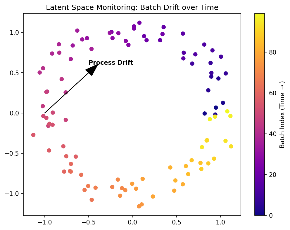
Materials example: process monitoring via latent drift

• Track latent embeddings \(\mathbf{z}_t\) over time during a manufacturing process.
• Drift from the normal cluster indicates process degradation.
• Advantage over raw sensor monitoring: latent space distills many sensors into a compact signal.
• Early drift detection enables preventive maintenance.

Process monitoring plot showing latent drift of production batches over time.

Lecture-essential vs exercise content split

• Lecture: latent space formalism, t-SNE/UMAP theory, kernel PCA, anomaly detection, trust quantification.
• Exercise: AE latent visualization, t-SNE and UMAP on Fashion MNIST, anomaly injection, comparison experiments.

Exercise setup summary

• Build AE on synthetic Gaussian pulse data; visualize 2D latent space.
• Apply t-SNE (sklearn) to Fashion MNIST subset; interpret the archipelago.
• Compare t-SNE vs UMAP: local vs global structure preservation.
• Inject anomalous signals; detect via reconstruction error and latent density.

Mini concept quiz

1. Which distribution is used in the low-dimensional space of t-SNE to solve the crowding problem?
   • 1. Gaussian distribution
   • 2. Uniform distribution
   • 3. Student-t distribution
   • 4. Poisson distribution
2. What is a key advantage of UMAP over t-SNE?
   • 1. It is slower but more accurate
   • 2. It better preserves global structure and supports transforming new data
   • 3. It only works for 2D visualization
   • 4. It does not have any hyperparameters
3. How is an anomaly typically identified in a trained autoencoder’s latent space?
   • 1. It maps to the center of the normal data cluster
   • 2. It has a very low reconstruction error
   • 3. It maps to a low-density region of the normal latent distribution
   • 4. It increases the training speed
4. What does “latent space interpolation” verify?
   • 1. The number of layers in the encoder
   • 2. The smoothness and continuity of the learned representation
   • 3. The exact value of the learning rate
   • 4. The rank of the input matrix

References + reading assignment for next unit

• Required reading before Unit 11:
  • Neuer: Ch. 5.5
  • McClarren: Ch. 4.4, 5
• Optional depth:
  • Murphy: Ch. 12 (latent linear models)
  • Bishop: Ch. 12 (kernel PCA)
• Next unit: Unsupervised Learning — clustering, mixture models, and density estimation.

Example Notebook

Week 10: Autoencoder Latent Space — IsingDataset (64×64)

Open rendered notebook →