Mathematical Foundations of AI & ML
Unit 11: Unsupervised Learning

Prof. Dr. Philipp Pelz

FAU Erlangen-Nürnberg

Title + Unit 11 positioning

• Units 9–10 explored learned representations and latent spaces.
• Unit 11: discovering structure in data without labels — the unsupervised paradigm.
• Core algorithms: K-Means clustering, Gaussian Mixture Models, and the EM algorithm.

Learning outcomes for Unit 11

By the end of this lecture, students can:

• state the K-Means objective and derive the assignment-update algorithm,
• formulate a GMM as a latent variable model,
• derive the E-step and M-step of EM for GMMs,
• explain why EM maximizes a lower bound on the log-likelihood.

Supervised vs unsupervised learning

Supervised

• Given input-output pairs \((\mathbf{x}_i, y_i)\)
• Learn the mapping \(f: X \to Y\)
• Direct teacher signal (labels)
• Goal: prediction/regression

Unsupervised

• Given inputs \(\mathbf{x}_i\) only
• Discover hidden structure
• No teacher signal
• Goal: pattern discovery

• Unsupervised learning is often a preprocessing step for supervised tasks.

Why unsupervised learning matters in engineering

• Labels are expensive: destructive testing (tensile strength), expert annotation (micrographs).
• Labels are unavailable: real-time sensor streams, exploratory data analysis.
• Labels are undefined: the goal is to discover unknown groupings or regimes.
• Unsupervised methods extract value from the vast amounts of unlabeled data in engineering.

Types of unsupervised learning

• Clustering: partition data into groups (K-Means, GMM).
• Density estimation: model the data distribution \(p(\mathbf{x})\).
• Dimensionality reduction: PCA, autoencoders (Units 2, 9–10).
• Generative models: learn to generate new samples similar to the data.
• Today: focus on clustering and density estimation via mixture models.

Clustering: the core task

• Partition \(N\) data points into \(K\) groups such that:
  • Within-group similarity is high (compact clusters).
  • Between-group similarity is low (separated clusters).
• The number of clusters \(K\) is typically a hyperparameter that must be chosen.

What defines a “good” cluster?

• Compact: low within-cluster variance.
• Separated: high distance between cluster centers.
• Interpretable: clusters correspond to meaningful categories.
• Different clustering objectives can produce different partitions of the same data.

Roadmap of today’s 90 min

• 10–25 min: K-Means algorithm — objective, convergence, initialization.
• 25–40 min: From hard to soft — GMM as probabilistic clustering.
• 40–55 min: EM algorithm — E-step, M-step, derivation.
• 55–70 min: Lower bound maximization and convergence guarantee.
• 70–80 min: Variants (K-Medoids, Bernoulli mixtures, model selection).
• 80–88 min: Engineering applications.

K-Means objective

• Minimize the total within-cluster sum of squared distances (distortion):

\[ J = \sum_{k=1}^{K} \sum_{i \in C_k} \|\mathbf{x}_i - \boldsymbol{\mu}_k\|^2 \]

• \(C_k\): set of points assigned to cluster \(k\). \(\boldsymbol{\mu}_k\): centroid of cluster \(k\).
• This is an NP-hard optimization problem — K-Means finds a local minimum [@neuer2024machine].

K-Means algorithm: two alternating steps

1. Assignment step: assign each point to the nearest centroid: \[ c_i = \arg\min_k \|\mathbf{x}_i - \boldsymbol{\mu}_k\|^2 \]

2. Update step: recompute centroids as the mean of assigned points: \[ \boldsymbol{\mu}_k = \frac{1}{|C_k|}\sum_{i \in C_k} \mathbf{x}_i \]

%%| fig-align: center
graph TD
    A[Initialize Centroids] --> B[Assign Points to Nearest Centroid]
    B --> C[Update Centroids to Mean of Assigned Points]
    C --> D{Convergence?}
    D -- No --> B
    D -- Yes --> E[Final Clusters]

• Repeat until assignments stop changing.

K-Means as coordinate descent

• The assignment step minimizes \(J\) with respect to cluster assignments (centroids fixed).
• The update step minimizes \(J\) with respect to centroids (assignments fixed).
• Each step reduces or maintains \(J\) — this is coordinate descent on the distortion cost.
• Since \(J\) is bounded below (by 0) and decreases monotonically, convergence is guaranteed.

K-Means convergence

• \(J\) decreases (or stays constant) at every step.
• There are finitely many possible assignments → algorithm must terminate.
• Convergence is to a local minimum — the result depends on initialization.
• Typical convergence: 10–50 iterations for moderate datasets [@mcclarren2021machine].

K-Means: initialization matters

• Random initialization can lead to poor local minima.
• K-Means++: choose first centroid randomly, then each subsequent centroid with probability proportional to squared distance from nearest existing centroid.
• Spreads initial centroids → much better results on average.
• Multiple restarts: run K-Means several times, keep the result with lowest \(J\).

K-Means: choosing K

• Elbow method: plot \(J\) vs \(K\). Look for the “elbow” where adding clusters gives diminishing returns.
• Silhouette score: for each point, compare within-cluster distance to nearest-neighbor-cluster distance. Average across all points.
• Domain knowledge: sometimes \(K\) is known (e.g., number of material phases).
• No universally best method — combine quantitative and qualitative assessment.

K-Means: limitations

• Assumes spherical clusters of roughly equal size and density.
• Hard assignments: each point belongs to exactly one cluster — no uncertainty.
• Sensitive to outliers (centroids pulled toward outliers).
• Cannot represent clusters with different shapes or orientations.
• These limitations motivate probabilistic clustering with GMMs.

K-Means: worked example

• 2D data with 3 Gaussian blobs (well-separated).
• Initialize: place 3 centroids (K-Means++).
• Iteration 1: assign points → update centroids.
• Iteration 5: centroids stabilize at cluster centers. Assignments are correct.
• Total distortion \(J\) decreases from ~150 to ~45 over 5 iterations.

K-Medoids: robust variant

• Instead of centroids (means), use actual data points as cluster representatives (medoids).
• Objective: minimize sum of distances (not necessarily squared) to nearest medoid.
• Robust to outliers: the medoid is a real data point, not pulled by extreme values.
• More expensive: \(O(N^2)\) per iteration vs \(O(NK)\) for K-Means.

Checkpoint: K-Means failure mode

• Question: K-Means splits a single elongated cluster into two halves. Why?
• Answer: K-Means assumes spherical clusters. An elongated cluster has high variance along one axis — two spherical clusters fit it better under the K-Means objective.
• Fix: use GMM with full covariance matrices.

From hard to soft clustering

Hard Clustering (K-Means)

• Each point belongs to exactly one cluster.
• Membership is binary: \(\{0, 1\}\).
• No representation of uncertainty.

Soft Clustering (GMM)

• Each point has a probability of belonging to each cluster.
• Membership is continuous: \([0, 1]\).
• Naturally handles overlap and uncertainty.

• Gaussian Mixture Models provide this probabilistic framework.

Gaussian Mixture Model: definition

\[ p(\mathbf{x}) = \sum_{k=1}^{K} \pi_k \, \mathcal{N}(\mathbf{x} | \boldsymbol{\mu}_k, \boldsymbol{\Sigma}_k) \]

• \(\boldsymbol{\pi}\): mixing coefficients (prior probability of cluster \(k\), \(\sum_k \pi_k = 1\)).
• \(\boldsymbol{\mu}_k\): mean of component \(k\).
• \(\boldsymbol{\Sigma}_k\): covariance of component \(k\) — allows elliptical clusters [@murphy2012machine].

GMM as a latent variable model

• Introduce a latent indicator \(z_i \in \{1, \dots, K\}\) for each data point:
  • \(p(z_i = k) = \pi_k\) (prior on cluster membership).
  • \(p(\mathbf{x}_i | z_i = k) = \mathcal{N}(\mathbf{x}_i | \boldsymbol{\mu}_k, \boldsymbol{\Sigma}_k)\).
• Marginalizing over \(z\) recovers the mixture: \(p(\mathbf{x}_i) = \sum_k \pi_k \mathcal{N}(\mathbf{x}_i | \boldsymbol{\mu}_k, \boldsymbol{\Sigma}_k)\).

Responsibilities: soft assignments

• The responsibility of cluster \(k\) for point \(i\) is the posterior:

\[ r_{ik} = p(z_i = k | \mathbf{x}_i) = \frac{\pi_k \, \mathcal{N}(\mathbf{x}_i | \boldsymbol{\mu}_k, \boldsymbol{\Sigma}_k)}{\sum_j \pi_j \, \mathcal{N}(\mathbf{x}_i | \boldsymbol{\mu}_j, \boldsymbol{\Sigma}_j)} \]

• \(r_{ik} \in [0, 1]\) and \(\sum_k r_{ik} = 1\) for each point \(i\).
• Responsibilities are the soft analogue of K-Means hard assignments.

The log-likelihood for GMMs

\[ \ell(\theta) = \sum_{i=1}^{N} \log \left[ \sum_{k=1}^{K} \pi_k \, \mathcal{N}(\mathbf{x}_i | \boldsymbol{\mu}_k, \boldsymbol{\Sigma}_k) \right] \]

• The sum inside the log makes direct optimization intractable.
• Setting derivatives to zero does not yield closed-form solutions.
• This motivates the EM algorithm as an iterative approach.

Why MLE is hard for mixtures

• The log of a sum cannot be decomposed into a sum of logs.
• The parameters \(\boldsymbol{\mu}_k, \boldsymbol{\Sigma}_k, \boldsymbol{\pi}\) are coupled through the responsibilities.
• Direct gradient-based optimization is possible but EM is more elegant and interpretable.
• EM decomposes the problem into tractable sub-problems.

The EM algorithm: overview

• Expectation-Maximization (Dempster, Laird & Rubin, 1977).
• A general algorithm for MLE in latent variable models.
• Two alternating steps:
  1. E-step: compute expected values of latent variables (responsibilities).
  2. M-step: maximize expected complete-data log-likelihood.

E-step: compute responsibilities

• Given current parameters \(\theta^{(t)} = \{\boldsymbol{\mu}_k, \boldsymbol{\Sigma}_k, \boldsymbol{\pi}^{(t)}\}\):

\[ r_{ik}^{(t)} = \frac{\pi_k^{(t)} \, \mathcal{N}(\mathbf{x}_i | \boldsymbol{\mu}_k^{(t)}, \boldsymbol{\Sigma}_k^{(t)})}{\sum_j \pi_j^{(t)} \, \mathcal{N}(\mathbf{x}_i | \boldsymbol{\mu}_j^{(t)}, \boldsymbol{\Sigma}_j^{(t)})} \]

• “Given the current model, how much does cluster \(k\) explain point \(i\)?”

M-step: update parameters

• Given responsibilities \(r_{ik}^{(t)}\), update parameters:

\[ N_k = \sum_{i=1}^{N} r_{ik}, \quad \boldsymbol{\mu}_k = \frac{1}{N_k}\sum_{i=1}^{N} r_{ik} \mathbf{x}_i \]

\[ \boldsymbol{\Sigma}_k = \frac{1}{N_k}\sum_{i=1}^{N} r_{ik} (\mathbf{x}_i - \boldsymbol{\mu}_k)(\mathbf{x}_i - \boldsymbol{\mu}_k)^\top, \quad \pi_k = \frac{N_k}{N} \]

• These are weighted versions of the sample statistics [@murphy2012machine].

EM algorithm: pseudocode

1. Initialize: set \(\boldsymbol{\mu}_k, \boldsymbol{\Sigma}_k, \boldsymbol{\pi}\) (e.g., from K-Means).
2. Repeat until convergence:
   • E-step: compute responsibilities \(r_{ik}\) for all \(i, k\).
   • M-step: update \(\boldsymbol{\mu}_k, \boldsymbol{\Sigma}_k, \boldsymbol{\pi}\) using weighted statistics.
   • Compute log-likelihood \(\ell(\theta)\).
3. Stop when \(\ell(\theta)\) changes by less than a threshold \(\epsilon\).

EM convergence

• Theorem: the log-likelihood \(\ell(\theta^{(t)})\) is non-decreasing: \(\ell(\theta^{(t+1)}) \geq \ell(\theta^{(t)})\).
• Convergence to a local maximum is guaranteed (not necessarily global).
• Rate of convergence depends on the “overlap” between components.
• Multiple restarts help find better local maxima.

The lower bound perspective

• EM can be understood as maximizing a lower bound on \(\ell(\theta)\).
• For any distribution \(q(z)\) over latent variables:

\[ \ell(\theta) \geq \sum_i \sum_k q(z_i = k) \log \frac{p(\mathbf{x}_i, z_i = k | \theta)}{q(z_i = k)} \]

• E-step: choose \(q = p(z|\mathbf{x}, \theta)\) to tighten the bound.
• M-step: maximize the bound w.r.t. \(\theta\) [@bishop2006pattern].

Jensen’s inequality and the auxiliary function

• Jensen’s inequality: \(\log \mathbb{E}[X] \geq \mathbb{E}[\log X]\) for concave \(\log\).
• The auxiliary function \(Q(\theta | \theta^{(t)}) = \mathbb{E}_{z|\mathbf{x},\theta^{(t)}}[\log p(\mathbf{x}, z | \theta)]\).
• M-step: \(\theta^{(t+1)} = \arg\max_\theta Q(\theta | \theta^{(t)})\).
• This guarantees \(\ell(\theta^{(t+1)}) \geq \ell(\theta^{(t)})\).

K-Means as a special case of EM

• Set all \(\boldsymbol{\Sigma}_k = \sigma^2 \mathbf{I}\) (isotropic, equal covariance).
• As \(\sigma \to 0\): responsibilities become hard (\(r_{ik} \to 0\) or \(1\)).
• E-step becomes the assignment step; M-step becomes the centroid update.
• K-Means is EM for a GMM with isotropic covariances in the zero-temperature limit.

GMM: worked example

• 2D data from 2 overlapping Gaussians (different means and covariances).
• Initialize from K-Means.
• E-step: points near boundaries get \(r_{ik} \approx 0.5\) (uncertain assignment).
• M-step: update means, covariances, mixing coefficients.
• After 10 iterations: log-likelihood converges; elliptical clusters correctly identified.

Checkpoint: EM understanding

• Question: After the E-step, what do the responsibilities tell you?
• Answer: The posterior probability of each cluster \(k\) given each data point \(\mathbf{x}_i\), under the current model parameters. They quantify how much each cluster “explains” each point.

Bernoulli mixture models

• For binary data (e.g., presence/absence of features):
  • Replace Gaussian with Bernoulli likelihood: \(p(\mathbf{x} | z = k) = \prod_j \mu_{kj}^{x_j}(1-\mu_{kj})^{1-x_j}\).
• EM updates: \(\mu_{kj} = \frac{\sum_i r_{ik} x_{ij}}{N_k}\) (weighted mean of binary features per cluster).
• Application: document clustering, genetic data analysis.

Model selection: choosing K

• BIC (Bayesian Information Criterion):

\[ \text{BIC} = \ell(\hat{\theta}) - \frac{K_{\text{params}}}{2}\log N \]

• AIC (Akaike Information Criterion):

\[ \text{AIC} = \ell(\hat{\theta}) - K_{\text{params}} \]

• Select \(K\) that maximizes BIC (or minimizes −BIC). Lower penalty = more components allowed.

BIC vs AIC

• BIC: stronger penalty for complexity (\(\log N / 2\) per parameter). Preferred for large \(N\).
• AIC: weaker penalty (1 per parameter). More permissive — tends to select larger \(K\).
• BIC is consistent (selects true \(K\) as \(N \to \infty\)). AIC is not.
• In practice: compare both and use domain knowledge to adjudicate.

Initialization strategies for EM

• Random: fast but unreliable — can converge to poor local maxima.
• K-Means: run K-Means first, use resulting centroids as initial means. Most common.
• Multiple restarts: run EM several times with different initializations, keep best log-likelihood.
• Good initialization is critical for EM convergence quality.

Singular covariance matrices

• If a cluster collapses to a single point, \(\boldsymbol{\Sigma}_k\) becomes singular (determinant = 0).
• The likelihood goes to infinity — a pathological solution.
• Fix: add a small diagonal regularization \(\boldsymbol{\Sigma}_k + \epsilon \mathbf{I}\).
• Alternative: constrain covariance matrices to be diagonal or shared across clusters.

Checkpoint: model selection

• Question: BIC selects \(K=3\) but you know there are 5 distinct groups. What might be wrong?
• Answer: The groups may significantly overlap, making them statistically indistinguishable. BIC prefers parsimony — 3 components may fit the data nearly as well as 5.

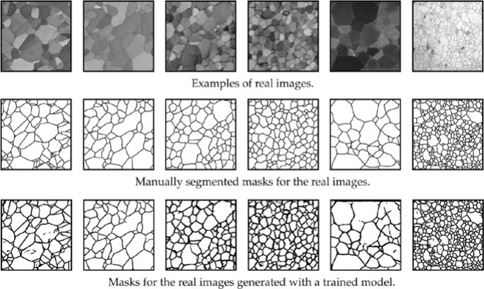
Application: image segmentation

• Model pixel colors (RGB) as a GMM with \(K\) components.
• Each component corresponds to a material or region (background, grain, defect).
• Segment the image by assigning each pixel to its most probable cluster.
• Soft assignments provide uncertainty at boundaries.

Unsupervised segmentation of polycrystalline microstructure.

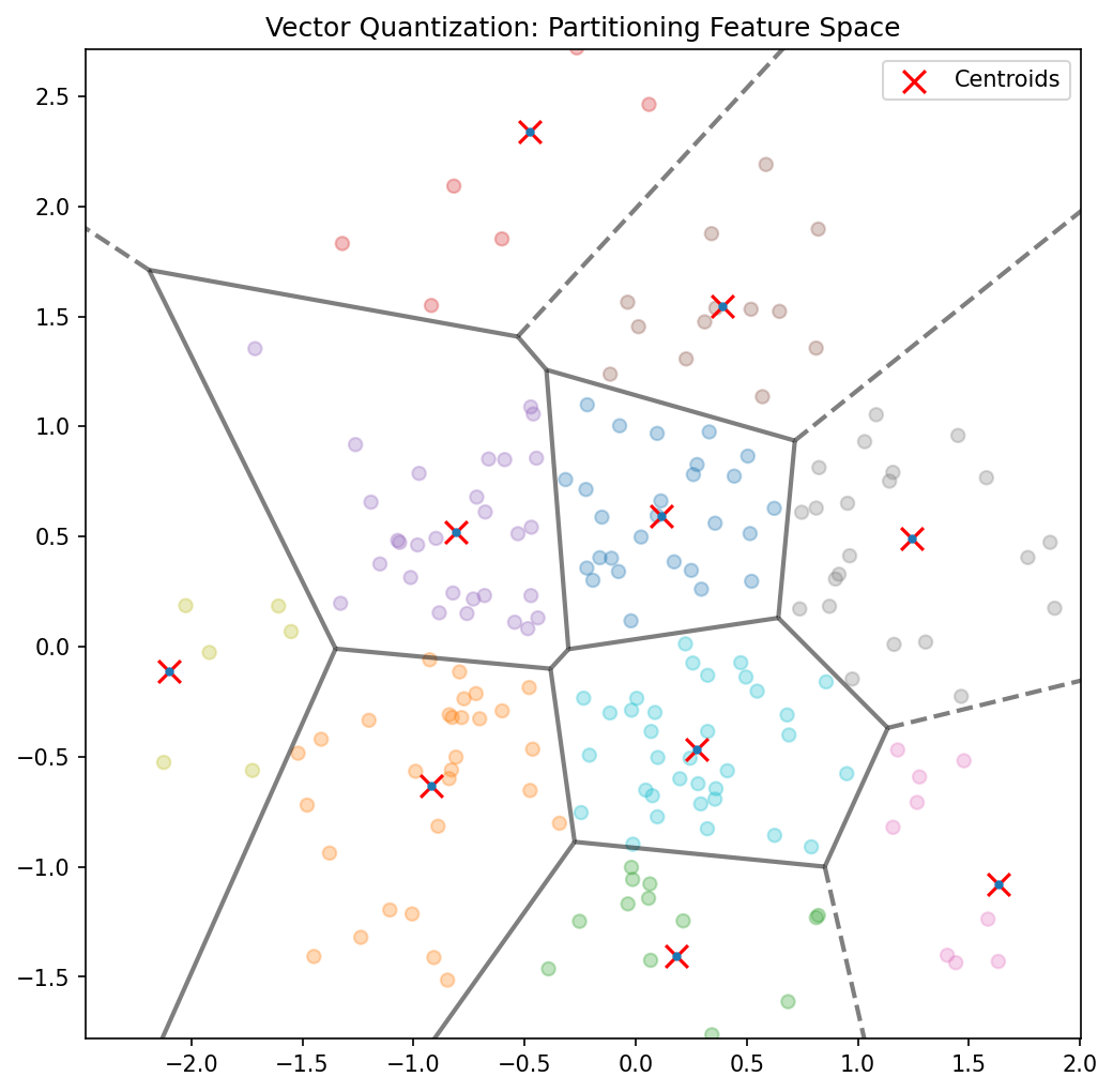
Application: vector quantization

• Replace each data point with its nearest centroid from a learned codebook.
• Used for signal compression: store cluster index instead of full data.
• Materials application: fingerprint alloy microstructures by their cluster assignments.
• Compression ratio = \(\log_2(\text{codebook size})\) bits per data point.

Vector quantization partitioning feature space into Voronoi cells.

Application: regime identification in manufacturing

• Cluster sensor data over time; each cluster represents an operating regime.
• Transitions between clusters indicate regime changes (startup, steady state, degradation).
• Real-time clustering enables automated process monitoring and control.

Placeholder: Time-series sensor data with clusters indicating different regimes

Application: anomaly detection via density

• Fit a GMM to normal operating data.
• For a new observation, compute \(p(\mathbf{x}_{\text{new}})\) under the GMM.
• Low density \(\to\) anomaly.
• This provides a principled, probabilistic anomaly score (unlike ad-hoc thresholds).

Clustering vs autoencoder embeddings

• Clustering operates in the original data space — affected by curse of dimensionality.
• Autoencoders provide a learned latent space where clustering may work better.
• Best of both: train autoencoder (Unit 9), then cluster in latent space.
• The latent space concentrates relevant variation, making cluster separation clearer.

Materials example: alloy phase identification

• Input: X-ray diffraction (XRD) patterns from unknown alloy samples.
• GMM clustering identifies distinct peak patterns → crystallographic phases.
• No prior labeling needed — the algorithm discovers phases from data.
• Responsibilities indicate mixed-phase samples (points between clusters).

Lecture-essential vs exercise content split

• Lecture: K-Means objective, GMM formulation, EM derivation, lower bound, model selection.
• Exercise: K-Means from scratch, EM for 2-component GMM, log-likelihood tracking, hard vs soft comparison.

Exercise setup summary

• Implement K-Means in NumPy on 2D synthetic Gaussian clusters.
• Implement EM for a 2-component GMM: responsibilities, parameter updates, log-likelihood.
• Compare K-Means hard assignments vs GMM soft assignments on overlapping clusters.
• Bonus: cluster autoencoder embeddings from Unit 10 and compare.

Exam-aligned summary: 10 must-know statements

1. K-Means minimizes within-cluster sum of squared distances.
2. K-Means alternates between assignment and update steps (coordinate descent).
3. A GMM models data as a weighted sum of Gaussian components.
4. Responsibilities are posterior probabilities of cluster membership.
5. The E-step computes responsibilities; the M-step updates parameters.
6. EM monotonically increases the log-likelihood (convergence to local max).
7. EM maximizes a lower bound on the observed-data log-likelihood.
8. K-Means is a limiting case of EM with isotropic covariances and hard assignments.
9. BIC/AIC balance model fit against complexity for choosing \(K\).
10. GMM-based density estimation enables principled anomaly detection.

References + reading assignment for next unit

• Required reading before Unit 12:
  • Murphy: Ch. 11.1–11.5
  • Neuer: Ch. 5.3
• Optional depth:
  • McClarren: Ch. 4.3 (K-Means)
  • Bishop: Ch. 9.2–9.4 (GMM and EM)
• Next unit: Uncertainty in Predictions — Bayesian predictive distributions and Gaussian Processes.

Example Notebook

Week 11: Unsupervised Clustering — NanoindentationDataset

Open rendered notebook →