Machine Learning in Materials Processing & Characterization
Unit 3: Data Quality, Preprocessing, and Robust Validation

Prof. Dr. Philipp Pelz

FAU Erlangen-Nürnberg

01. The Quality Crisis in Scientific ML

• Garbage In, Garbage Out: An algorithm is only as good as the data it sees
• In materials science, data is expensive — so we tend to use everything, even the “garbage”
• The Reproducibility Crisis: Many published models fail on new samples

Note

Unit 3 focuses on everything that happens before and after modeling — the steps most often skipped.

02. Learning Outcomes

By the end of this unit, you can:

1. Design a systematic data cleaning pipeline for lab data
2. Choose appropriate scaling/normalization for different feature types
3. Identify and prevent the three types of data leakage
4. Apply K-fold and grouped cross-validation correctly
5. Select appropriate error metrics for regression and classification
6. Evaluate model reliability beyond simple accuracy

03. The ML Workflow: Where Are We?

graph LR
    C["Collection"] --> PP["Preprocessing"]
    PP --> M["Modeling"]
    M --> E["Evaluation"]
    E --> D["Deployment"]
    style PP fill:#e7ad52,color:#000
    style E fill:#e7ad52,color:#000

Today we focus on the gold boxes: Preprocessing and Evaluation.

These are where 80% of the work happens — and where 80% of the mistakes hide.

04. The Role of Preprocessing

Transforming raw, potentially messy data into a structured format suitable for algorithms:

• Raw sensor readings → clean feature matrix
• Inconsistent units → standardized scales
• Missing values → complete records (or honest gaps)
• Artifacts → detected and documented

Part 1: Data Cleaning

Slides 05–11

05. Common Data Issues

• Structural problems: Typos in labels, mixed units (mm vs. µm), inconsistent naming
• Duplicates: Same measurement recorded twice — inflates dataset and biases training
• Irrelevant observations: Test runs, calibration samples left in the dataset
• Missing values (NaNs): Sensor failure, transmission drops, out-of-range readings
• Outliers: Extreme values — physical or artifactual?

06. Missing Values: Sources and Detection

Why data goes missing:

• Sensor failure during measurement
• Transmission dropout (wireless sensors)
• “Out of range” readings clipped by the instrument
• Operator error (forgot to record a parameter)

Detection: df.isnull().sum() in Pandas — always the first thing to check.

07. Handling Missing Values

Fix at source (ideal):

• Repair the sensor
• Re-run the measurement
• Check the raw data files

Digital repair (if source fix impossible):

• Deletion: Remove rows/columns (wasteful for small data)
• Interpolation: Linear, spline for time-series
• Imputation: Mean/median (dangerous for multi-modal data)
• Physics-based: Fill using conservation laws

Numerical markers: Using “impossible” values (e.g., -1000°C) to track NaNs without losing record count.

08. Outlier Detection

Three types of outliers:

• Point (global): A single value far from the distribution (e.g., hardness = 5000 HV)
• Contextual: Normal globally but unusual in context (e.g., 200°C during a room-temperature test)
• Collective: A group that behaves differently from the rest (e.g., an entire batch with drift)

09. Think About This: To Remove or Not?

Scenario: You find a hardness value 3× higher than all others in your dataset.

• 1. Remove it — it’s clearly an error
• 2. Keep it — it might be real (e.g., a hard precipitate)
• 3. Investigate — check the measurement log before deciding

Answer: Always (C). Is it a cosmic ray on the detector? A typo? Or a rare but real physical event (crack initiation, phase transformation)?

Removing real outliers destroys the most interesting data points.

10. Duplicate Tracking

• Redundant data points bias training (over-weighting certain conditions)
• Duplicates between train and test sets cause leakage
• Sources: Copy-paste errors, merging overlapping databases, augmentation artifacts

# Simple duplicate check
n_duplicates = df.duplicated().sum()
print(f"Found {n_duplicates} duplicate rows")
df = df.drop_duplicates()

11. The Systematic Cleaning Pipeline

1. Detection: Identify outliers, NaNs, duplicates, structural issues
2. Diagnosis: Is the issue physical or artifactual? Check the measurement log
3. Treatment: Delete, cap, impute, or flag — with justification
4. Documentation: Always report how much data was altered!

Note

If you remove 20% of your data without documenting why, your results are not reproducible.

Part 2: Data Transformation and Scaling

Slides 12–20

12. Why Transform Data?

• Linearize trends: Log-transform for exponential relationships
• Align features: Temperature in [20, 1200] vs. composition in [0.01, 0.5]
• Equal weighting: Algorithms using distance (kNN, SVM) need comparable scales
• Numerical stability: Very large or very small values cause floating-point issues

13. Centering and Shifting

• Mean centering: \(x' = x - \bar{x}\) (center at zero)
• Required for covariance-based methods (PCA, correlation analysis)
• Peak alignment: Shifting spectra so that a reference peak is at position zero

Centering changes the origin but not the shape or spread of the distribution.

14. Min-Max Scaling

\[x' = \frac{x - x_{\min}}{x_{\max} - x_{\min}} \in [0, 1]\]

• Maps all features to the same range
• Weakness: Sensitive to outliers — one extreme value stretches the entire scale

Good for: Neural network inputs (bounded activations like sigmoid expect [0,1]).

Bad for: Noisy lab data with occasional extreme values.

15. Standardization (Z-score)

\[x' = \frac{x - \mu}{\sigma}\]

• Mean = 0, Standard deviation = 1
• Robust to differences in feature magnitude
• The default choice for most ML algorithms

from sklearn.preprocessing import StandardScaler
scaler = StandardScaler()
X_train_scaled = scaler.fit_transform(X_train)  # Fit on training only!
X_test_scaled = scaler.transform(X_test)         # Apply to test

16. Robust Scaler

\[x' = \frac{x - \text{median}}{\text{IQR}}\]

• Uses median and interquartile range instead of mean and std
• Best for noisy lab data: Outliers don’t distort the scaling
• Available as sklearn.preprocessing.RobustScaler

17. Log-Transforms

• Useful for variables spanning several orders of magnitude:
  • Grain sizes: 0.1 µm to 1000 µm
  • Dislocation densities: \(10^6\) to \(10^{15}\) m\(^{-2}\)
• Linearizes exponential trends → simpler models work better

Caution: Log-transform requires strictly positive values. Check for zeros first!

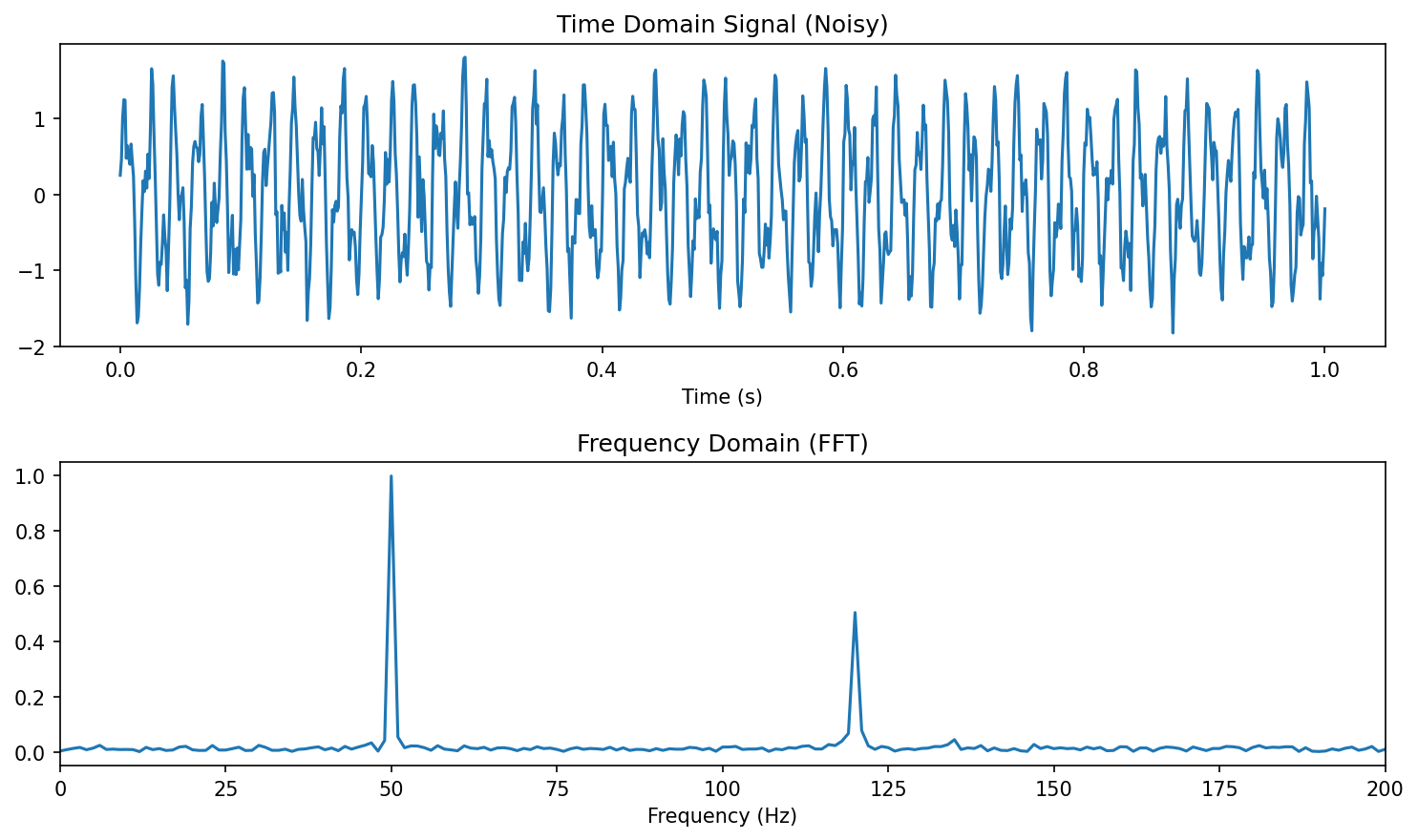
18. Frequency Domain: FFT

• Fast Fourier Transform: Convert time-domain → frequency-domain
• Detect oscillations, periodicity, and characteristic frequencies
• Materials example: Vibration analysis during milling → tool wear detection

19. Wavelet Transforms: Time-Frequency Analysis

• FFT loses when frequencies occur — Wavelets keep both time and frequency
• Localizing features that are both temporal and periodic
• Materials example: Acoustic emission during crack propagation — the frequency signature changes over time

20. Triggering: Isolating Relevant Sequences

• Long time series often contain mostly irrelevant data
• Triggering: Automatically extracting relevant windows
  • Example: Isolating loading cycles from a continuous fatigue test
  • Example: Extracting melting events from a continuous temperature log

Critical rule for all transformations: Scalers and transforms must be “fit” on training data only and “applied” to test data. Otherwise: preprocessing leakage.

Part 3: Labeling and Uncertainty

Slides 21–24

21. The Annotation Problem

• Who provides the “Ground Truth”?
• In microscopy, labeling is manual and tedious: drawing grain boundaries, identifying phases, marking defects
• Label uncertainty: If two experts disagree, which one is “right”?

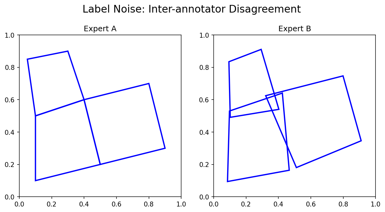
22. Inter-Annotator Variance

• Different experts segment the same micrograph differently
• This variance sets an upper bound on meaningful model performance
• If humans only agree 85% of the time, a model claiming 99% accuracy is likely overfitting to one person’s bias

Best practice: Have multiple annotators. Report the inter-annotator agreement. Your model should aim for human-level performance, not perfect accuracy.

23. Quantifying Label Uncertainty

• Models shouldn’t just output a label — they should output confidence
• Softmax probabilities: \(P(\text{Phase} = \text{FCC}) = 0.82\)
• Confidence < 0.6? The model is uncertain — flag for expert review

The Bayesian perspective: treat model parameters as distributions, not point estimates. Prior + Likelihood = Posterior.

24. Active Learning: Smart Annotation

• Instead of labeling everything, the model asks: “Label this specific image because I am most uncertain about it”
• Reduces manual burden while focusing on the “hard” physical cases

graph LR
    U["Unlabeled<br>Pool"] --> M["Model<br>Predicts"]
    M --> Q["Query:<br>Most Uncertain"]
    Q --> E["Expert<br>Labels"]
    E --> T["Retrain<br>Model"]
    T --> M

Part 4: Robust Validation and Model Selection

Slides 25–37

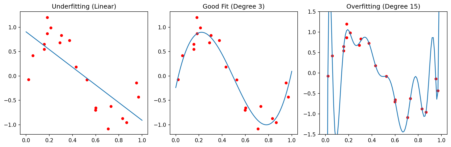
25. Overfitting vs. Underfitting

Underfitting (High Bias):

• Model is too simple
• Fails to capture the trend
• High error on both train and test

Overfitting (High Variance):

• Model is too complex
• Memorizes noise as if it were signal
• Low train error, high test error

26. The Bias-Variance Tradeoff

\[\text{Total Error} = \text{Bias}^2 + \text{Variance} + \text{Irreducible Noise}\]

• Bias: Error from wrong assumptions (model too simple)
• Variance: Error from sensitivity to training data (model too complex)
• Irreducible noise: Aleatory uncertainty — the noise floor

The sweet spot: enough complexity to capture the physics, not so much that you memorize the noise.

27. Parsimony and Regularization

Occam’s Razor: Prefer the simplest model that explains the data.

“Entities must not be multiplied beyond necessity.”

Regularization adds a penalty for complexity:

• L1 (Lasso): \(J = \text{MSE} + \lambda \sum |w_i|\) — can force weights to exactly zero (feature selection!)
• L2 (Ridge): \(J = \text{MSE} + \lambda \sum w_i^2\) — shrinks weights toward zero

28. Train-Test Split (Holdout)

• Divide data into independent sets:
  • Training set (70-80%): Learn model parameters
  • Test set (20-30%): Evaluate final performance
• The test set must never influence training decisions

Risk for small datasets: An unlucky split puts all “hard” cases in the test set → pessimistic estimate. Or all “easy” cases → optimistic estimate.

29. K-Fold Cross-Validation

• Split data into \(K\) folds (typically \(K = 5\) or \(10\))
• Iteratively use \(K-1\) folds for training, 1 for testing
• Average the \(K\) performance scores

graph TD
    D["Dataset"] --> F1["Fold 1: Test"]
    D --> F2["Fold 2: Test"]
    D --> F3["Fold 3: Test"]
    D --> F4["Fold 4: Test"]
    D --> F5["Fold 5: Test"]
    F1 --> A["Average<br>Performance"]
    F2 --> A
    F3 --> A
    F4 --> A
    F5 --> A

More stable than holdout: every sample gets to be in the test set exactly once.

30. Leave-One-Out (LOOCV)

• Special case: \(K = N\) (number of samples)
• Each sample is tested individually against a model trained on all others
• Most robust for very small datasets (\(N < 50\))
• Most expensive computationally: train \(N\) models

31. Stratified Splitting

• Ensure each fold has the same class distribution as the full dataset
• Crucial for imbalanced data: if only 5% of samples are “defective,” a random fold might contain zero defective samples

from sklearn.model_selection import StratifiedKFold
skf = StratifiedKFold(n_splits=5, shuffle=True)
for train_idx, test_idx in skf.split(X, y):
    # Each fold has same proportion of each class
    ...

32. Data Leakage: The Silent Killer

Definition: When information from the test set “leaks” into training, producing over-optimistic results that vanish during real deployment.

Three types of leakage in materials ML:

1. Spatial/Group leakage: Patches from the same sample in train and test
2. Temporal leakage: Using future data to predict the past
3. Preprocessing leakage: Fitting scalers on the full dataset

Note

“If your accuracy is too good to be true, it probably is.”

33. Spatial/Group Leakage

Scenario: A sample is cut into 100 image patches. 80 go to train, 20 to test.

Problem: Patches from the same physical sample are highly correlated. The model “recognizes” the specific sample instead of learning general physics.

Solution: Split by Sample ID or Batch ID, never by patch.

from sklearn.model_selection import GroupKFold
gkf = GroupKFold(n_splits=5)
for train_idx, test_idx in gkf.split(X, y, groups=sample_ids):
    ...

34. Temporal Leakage

Scenario: Predict the quality of a weld based on sensor logs.

Problem: Using data from \(t = 50\) min to predict a property measured at \(t = 10\) min.

Solution: “Walk-forward” validation — only use data available at the time of prediction.

In time-series: never shuffle! The arrow of time must be respected in your splits.

35. Preprocessing Leakage

Scenario: Calculate mean and standard deviation of the entire dataset before splitting.

Problem: Information about the test set distribution is now embedded in the training features.

Solution: Use Pipeline objects to encapsulate all preprocessing.

from sklearn.pipeline import Pipeline
pipe = Pipeline([
    ('scaler', StandardScaler()),  # Fit only on training fold
    ('model', LinearRegression())
])
cross_val_score(pipe, X, y, cv=GroupKFold(5), groups=sample_ids)

36. Think About This: Spot the Leakage

Setup: You have 20 steel samples. Each is imaged at 5 locations. You standardize all features, then randomly split the 100 images into 80 train / 20 test. You achieve R² = 0.95.

How many leakage errors are present?

Answer: Three!

1. Preprocessing leakage: Standardization before splitting
2. Spatial leakage: Images from the same sample in train and test
3. No grouped validation: Should split by sample ID, not by image

37. Nested Cross-Validation

• Outer loop: Evaluates model performance (5-fold)
• Inner loop: Tunes hyperparameters (5-fold within each outer fold)
• Prevents hyperparameter tuning from biasing the performance estimate

Computationally expensive (\(5 \times 5 = 25\) model fits) but the gold standard for small datasets.

Part 5: Error Measures

Slides 38–47

38. Measuring Success: Which Metric?

• Different tasks need different measures
• A metric defines what “good” means — choose it as carefully as your model

Task	Common Metrics
Regression	MAE, MSE, RMSE, R²
Classification	Accuracy, Precision, Recall, F1, AUC
Segmentation	IoU (Jaccard), Dice, Pixel Accuracy

39. Regression: MAE (L1 Error)

\[\text{MAE} = \frac{1}{N}\sum_{i=1}^{N} |y_i - \hat{y}_i|\]

• Mean Absolute Error — in the original units of the target
• Less sensitive to outliers than MSE
• Interpretable: “On average, our prediction is off by X MPa”

40. Regression: MSE, RMSE (L2 Error)

\[\text{MSE} = \frac{1}{N}\sum_{i=1}^{N} (y_i - \hat{y}_i)^2 \qquad \text{RMSE} = \sqrt{\text{MSE}}\]

• MSE: Penalizes large errors disproportionately (quadratic)
• RMSE: Returns to original units — comparable to MAE
• Use MSE when large errors are especially bad (safety-critical applications)

41. Regression: R² (Coefficient of Determination)

\[R^2 = 1 - \frac{\sum(y_i - \hat{y}_i)^2}{\sum(y_i - \bar{y})^2}\]

• Fraction of variance “explained” by the model
• \(R^2 = 1\): perfect fit. \(R^2 = 0\): model is no better than predicting the mean
• \(R^2 < 0\) is possible: model is worse than the mean!

Pitfall: High R² doesn’t mean a useful model. Always check residual plots.

42. Classification: The Confusion Matrix

	Predicted Positive	Predicted Negative
Actually Positive	TP (True Positive)	FN (False Negative)
Actually Negative	FP (False Positive)	TN (True Negative)

• Type I Error (FP): “Crying wolf” — predicting a defect that isn’t there
• Type II Error (FN): “Missing the wolf” — missing a real defect
• Which is worse depends on the application!

43. Precision: Avoiding False Alarms

\[\text{Precision} = \frac{TP}{TP + FP}\]

“Of all predicted positives, how many were actually positive?”

Materials example: Automated defect detection in a production line.

High precision = few false alarms → operators trust the system.

44. Recall (Sensitivity): Finding Everything

\[\text{Recall} = \frac{TP}{TP + FN}\]

“Of all actually positive cases, how many did we find?”

Materials example: Safety-critical inspection of turbine blades.

High recall = we find (almost) every crack → no catastrophic failures.

45. F1-Score: Balancing Precision and Recall

\[F_1 = 2 \cdot \frac{\text{Precision} \cdot \text{Recall}}{\text{Precision} + \text{Recall}}\]

• Harmonic mean of precision and recall
• F1 = 1 only if both precision and recall are perfect
• Also known as the Dice coefficient in image segmentation

46. IoU (Jaccard Similarity)

\[\text{IoU} = \frac{|A \cap B|}{|A \cup B|} = \frac{TP}{TP + FP + FN}\]

• Intersection over Union: Standard for image segmentation and object detection
• Stricter than Dice: penalizes both false positives and false negatives
• IoU > 0.5 is a common threshold for “acceptable” segmentation

47. Categorical Cross-Entropy

\[L = -\sum_{c=1}^{C} y_c \log(\hat{y}_c)\]

• The standard loss function for multi-class classification
• Penalizes incorrect high-confidence predictions heavily
• Used during training (not as an evaluation metric)

Connection: Cross-entropy is the negative log-likelihood under a categorical distribution — it’s the Bayesian-correct loss for classification.

Summary and Key Takeaways

Slides 48–50

48. Summary: Preprocessing

1. Clean your data — but fix the physics first (source correction > digital repair)
2. Scale appropriately: Z-score by default, RobustScaler for noisy data
3. Transform thoughtfully: Log, FFT, wavelets — match the physics
4. Document everything: A cleaning log is part of your reproducibility

49. Summary: Validation and Metrics

1. Human labels are uncertain → quantify disagreement, don’t chase 100% accuracy
2. Beware of leakage → split by sample, not by pixel; respect the arrow of time
3. Cross-validate properly → grouped K-fold + nested CV for hyperparameters
4. Choose the right metric → what matters in your application? Safety? Cost? Trust?

50. The Trustworthy Materials ML Checklist

• Is my split leakage-safe (grouped by sample)?
• Did I fit the scaler only on the training set?
• Do my labels have an uncertainty estimate?
• Is my metric sensitive to class imbalance?
• Have I benchmarked against a simple baseline?
• Are my residuals random (no systematic pattern)?
• Can someone reproduce my preprocessing from my documentation?

Reading:

• Neuer (2024): Ch. 3 (Data Preprocessing) (Neuer et al. 2024)
• Sandfeld (2024): Ch. 11.5, 16.2 (Validation) (Sandfeld et al. 2024)
• McClarren (2021): Ch. 1, 3 (Evaluation and Metrics) (McClarren 2021)

Next Week: Unit 4 — From Classical Microstructure Metrics to Learned Representations

References

McClarren, Ryan G. 2021. Machine Learning for Engineers: Using Data to Solve Problems for Physical Systems. Springer.

Neuer, Michael et al. 2024. Machine Learning for Engineers: Introduction to Physics-Informed, Explainable Learning Methods for AI in Engineering Applications. Springer Nature.

Sandfeld, Stefan et al. 2024. Materials Data Science. Springer.