Machine Learning in Materials Processing & Characterization
Unit 5: Convolutional Neural Networks for Microstructure Analysis

Prof. Dr. Philipp Pelz

FAU Erlangen-Nürnberg

01. From Vectors to Images

• Last week: Multi-Layer Perceptrons (MLPs) for tabular data
• This week: Convolutional Neural Networks (CNNs) for images
• Why can’t we just use a standard MLP for a micrograph?

The problem: Images have spatial structure that MLPs destroy.

02. Learning Outcomes

By the end of this unit, you can:

1. Explain why MLPs fail for high-resolution images (parameter explosion)
2. Define convolution, kernels, stride, and padding
3. Explain local connectivity, weight sharing, and translation invariance
4. Distinguish between Max and Average Pooling
5. Describe key CNN architectures (LeNet, AlexNet, ResNet, U-Net)
6. Apply CNN concepts to microstructure segmentation and classification

Section 1: The Image Problem

Slides 03–08

03. Microscopy Data is Inherently Spatial

Materials characterization produces diverse image data:

• SEM: Surface morphology (µm resolution)
• TEM: Atomic structure (Å resolution)
• AFM: Surface topography (nm resolution)
• Optical: Macro-scale structure (µm–mm)

All share a common property: nearby pixels are correlated — physics ensures spatial continuity.

04. The Parameter Explosion (I)

Example: A modest \(64 \times 64\) image

• Input size: \(64 \times 64 = 4{,}096\) pixels
• One hidden layer with 512 neurons
• Parameters: \(4{,}096 \times 512 = \mathbf{2.1 \text{ million}}\) weights

This is already large. But real micrographs are much bigger…

05. The Parameter Explosion (II)

Realistic example: A \(1024 \times 1024\) SEM image

• Input size: \(1{,}048{,}576\) pixels
• One hidden layer with 512 neurons
• Parameters: \(1{,}048{,}576 \times 512 = \mathbf{537 \text{ million}}\) weights
• Memory: ~4 GB just for one layer!

Note

With only 100 training images, a 537M parameter model will memorize every sample perfectly — and generalize to nothing.

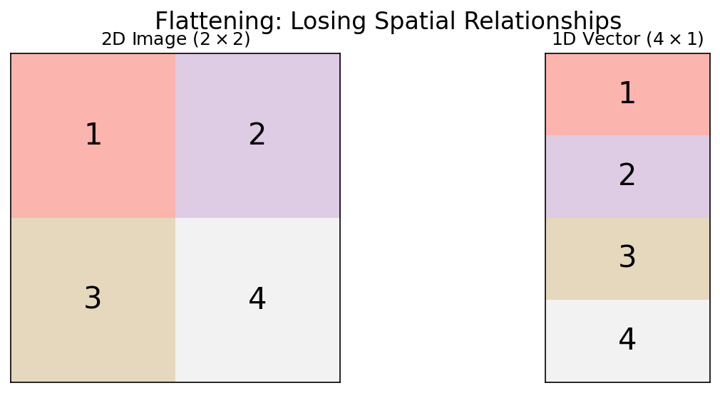
06. Loss of Spatial Structure

• MLPs flatten images into 1D vectors: pixel (0,0), pixel (0,1), …
• Result: Neighboring pixels (same grain) are treated identically to distant pixels (different phases)
• The spatial correlation — the key physical information — is destroyed

07. The Translation Problem

• If a precipitate moves 5 pixels to the right, the MLP sees a completely different input pattern
• It must relearn the precipitate at every possible position
• This is hopelessly wasteful — the same feature appears everywhere in the image

What we want: A feature detector that works the same way regardless of position — translation invariance.

08. Section 1 Recap

1. Microscopy images have spatial structure that encodes physics
2. MLPs suffer a parameter explosion on high-resolution images
3. Flattening destroys spatial relationships
4. We need translation-invariant feature detection
5. The solution: Convolutional Neural Networks

Section 2: The Convolution Layer

Slides 09–20

09. Convolution: The Core Idea

• Slide a small “window” (kernel/filter) over the image
• At each position, compute a weighted sum
• The output is a feature map: a new image highlighting specific patterns

graph LR
    I["Input Image"] --> K["Kernel<br>(3×3)"]
    K --> FM["Feature Map<br>(detected edges)"]

10. The Discrete Convolution Formula

\[(I * K)_{m,n} = \sum_{i}\sum_{j} I_{m-i,\, n-j} \cdot K_{i,j}\]

• \(I\): input image
• \(K\): kernel (filter) — typically \(3 \times 3\) or \(5 \times 5\)
• The kernel slides across the image, computing element-wise products and summing

11. Visualizing the Sliding Window

• Input: \(5 \times 5\) image
• Kernel: \(3 \times 3\)
• Output: \(3 \times 3\) feature map (without padding)
• Each output pixel “sees” a \(3 \times 3\) local neighborhood

12. The Feature Map

• The output of one convolution is called a feature map
• Each pixel in the feature map represents how strongly the kernel’s pattern was detected at that location
• High values = strong match. Low values = weak match.

A single kernel produces one feature map. We use multiple kernels to detect multiple features simultaneously.

13. Kernels as Feature Detectors (I)

Edge detection (Laplacian):

\[K = \begin{pmatrix} 0 & -1 & 0 \\ -1 & 4 & -1 \\ 0 & -1 & 0 \end{pmatrix}\]

Highlights boundaries between regions.

Blur (Gaussian):

\[K = \frac{1}{16}\begin{pmatrix} 1 & 2 & 1 \\ 2 & 4 & 2 \\ 1 & 2 & 1 \end{pmatrix}\]

Smooths noise by averaging neighbors.

14. Kernels as Feature Detectors (II)

Horizontal edges: \[K_h = \begin{pmatrix} -1 & -1 & -1 \\ 0 & 0 & 0 \\ 1 & 1 & 1 \end{pmatrix}\]

Vertical edges: \[K_v = \begin{pmatrix} -1 & 0 & 1 \\ -1 & 0 & 1 \\ -1 & 0 & 1 \end{pmatrix}\]

In a CNN: The network discovers that these filters (and many others) are useful for the task — automatically, from data.

15. Stride: Controlling the Step Size

• Stride = how many pixels the kernel moves at each step
• Stride 1: kernel moves one pixel → output nearly same size as input
• Stride 2: kernel moves two pixels → output is half the size

Higher stride = faster computation, lower resolution output. A design trade-off.

16. Padding: Preserving Image Size

• Without padding, a \(3 \times 3\) kernel on a \(W \times W\) image produces \((W-2) \times (W-2)\)
• Images shrink after each convolution!

• “Valid” padding: No padding, output shrinks
• “Same” padding: Add zeros at borders → output size = input size
• Same padding is the standard in most architectures

17. Think About This: Parameter Savings

Compare: Processing a \(1024 \times 1024\) image

Approach	Parameters
MLP (512 hidden units)	537 million
One \(3 \times 3\) conv filter	9
64 conv filters	576

That’s a 930,000× reduction! Weight sharing is the key: the same 9 weights are reused at every position in the image.

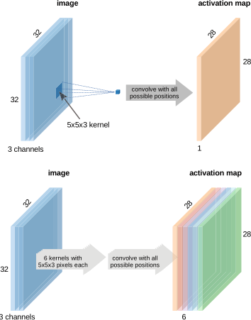
18. Multi-Channel Convolution

• Real images have depth (channels):
  • Grayscale: 1 channel
  • RGB: 3 channels
  • Hyperspectral: 100+ channels
  • Feature maps from previous layer: \(C\) channels

A kernel on multi-channel input has shape \(C \times k \times k\). It sums across all channels.

19. Activation in CNNs

After each convolution, apply a non-linear activation:

\[\text{Feature Map} = \text{ReLU}(I * K + b)\]

• ReLU keeps only positive activations: “this feature is present here”
• Same activation functions as in MLPs (Unit 4)

20. Section 2 Recap

1. Convolution = sliding a kernel over the image, computing local weighted sums
2. Kernels are feature detectors (edges, textures, blobs)
3. Stride controls spatial downsampling; padding preserves size
4. Weight sharing reduces parameters by 5-6 orders of magnitude vs. MLPs
5. Multi-channel convolution enables combining features across depth

Section 3: Architectural Principles

Slides 21–30

21. Local Connectivity

• Each neuron in a conv layer “sees” only a small local patch of the input
• A \(3 \times 3\) kernel means each output pixel depends on only 9 input pixels
• Physical justification: Features in micrographs are local (grain boundaries, precipitates)

22. Weight Sharing

• The same kernel is used at every spatial position
• One set of weights → applied millions of times
• Assumption: A feature that’s useful in one part of the image is useful everywhere

Note

Weight sharing encodes translation invariance into the architecture — we don’t need to learn the same feature at every position.

23. Translation Invariance vs. Equivariance

Translation Equivariance:

If the input shifts, the feature map shifts by the same amount.

Conv layers are equivariant.

Translation Invariance:

The output doesn’t change when the input shifts.

Classification layers (after pooling + flattening) are invariant.

Equivariance preserves “where” the feature is. Invariance discards “where” and keeps only “what.”

24. The Concept of Depth

• Each conv layer has multiple filters → multiple feature maps
• The number of filters per layer is called the layer’s “depth” or “channels”
• Typical progression: 64 → 128 → 256 → 512 channels

More filters = more features detected. But also more parameters and computation.

25. The Receptive Field (I)

• Receptive field: The region of the input image that influences a specific output neuron
• A single \(3 \times 3\) conv layer: receptive field = \(3 \times 3\)
• Two stacked \(3 \times 3\) layers: receptive field = \(5 \times 5\)
• Three stacked layers: receptive field = \(7 \times 7\)

26. The Receptive Field (II)

With stride and pooling, the receptive field grows faster:

\[r_{\text{eff}} = r + (k - 1) \times \prod_{i} s_i\]

where \(k\) is kernel size and \(s_i\) are strides of preceding layers.

Design rule: The receptive field should be large enough to “see” the features you want to detect. Grain boundary detection needs at least grain-sized receptive fields.

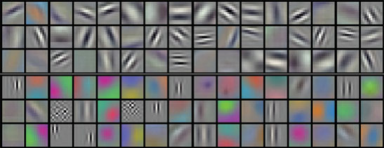
27. The Hierarchy of Features

• Layer 1: Simple edges, dots, intensity gradients
• Layer 2: Textures, corners, simple shapes (grain boundary segments)
• Layer 3: Complex morphologies (dendrites, twins, precipitate clusters)
• Final layers: Global material state or classification

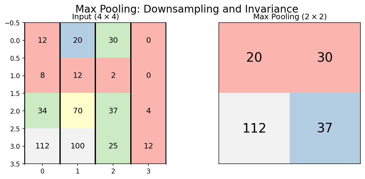
28. Full CNN Anatomy

graph LR
    I["Input<br>Micrograph"] --> C1["Conv + ReLU<br>(64 filters)"]
    C1 --> P1["MaxPool<br>(2×2)"]
    P1 --> C2["Conv + ReLU<br>(128 filters)"]
    C2 --> P2["MaxPool<br>(2×2)"]
    P2 --> C3["Conv + ReLU<br>(256 filters)"]
    C3 --> F["Flatten"]
    F --> FC["FC Layers"]
    FC --> O["Output<br>(Phase A/B)"]

1. Feature Extractor: Alternating Conv + Pooling layers
2. Classifier: Flatten → Fully Connected → Output

29. Think About This: Designing a CNN

Task: You need to classify microstructure images as “martensitic” or “ferritic.” Your images are \(256 \times 256\) grayscale. You have 200 labeled images.

What’s your concern?

Answer: 200 images is far too few to train a CNN from scratch. Even a modest CNN has millions of parameters. You’ll need transfer learning (Unit 6) or data augmentation. Start with the simplest possible model.

30. Section 3 Recap

1. Local connectivity: Each neuron sees only a small patch
2. Weight sharing: Same kernel everywhere → massive parameter reduction
3. Translation equivariance/invariance: Features detected regardless of position
4. Receptive field: Grows with depth — must match feature scale
5. Feature hierarchy: Edges → textures → morphologies → classification

Section 4: The Pooling Layer

Slides 31–38

31. Why Pool?

• Downsampling: Reduce spatial dimensions → less computation
• Noise robustness: Small pixel shifts don’t change the output
• Increase receptive field: Each pixel in the pooled output covers a larger input region

32. Max Pooling

• Take the maximum value in each window (typically \(2 \times 2\))
• Preserves the strongest signal in each region
• Spatial size: halved in each dimension

\[\text{MaxPool}(x)_{m,n} = \max_{i,j \in \text{window}} x_{m+i, n+j}\]

33. Average Pooling

• Take the mean value in each window
• Preserves the overall signal level
• Less aggressive than max pooling — retains more information about intensity

\[\text{AvgPool}(x)_{m,n} = \frac{1}{|W|}\sum_{i,j \in \text{window}} x_{m+i, n+j}\]

Used more often in later layers. Global Average Pooling (over the entire feature map) is standard for the final layer of modern architectures.

34. Pooling and Shift Invariance

• If the input shifts by 1 pixel, the feature map shifts by 1 pixel
• After \(2 \times 2\) max pooling: a 1-pixel shift may produce the same output
• Pooling provides approximate translation invariance

Materials implication: A precipitate at pixel (50, 50) and one at pixel (51, 51) produce the same classification — which is physically correct.

35. The Conv-Pool Block

The standard building block of CNNs:

\[\text{Input} \xrightarrow{\text{Conv}} \xrightarrow{\text{ReLU}} \xrightarrow{\text{Pool}} \text{Output}\]

Typically repeated 3-5 times, with increasing filter count:

Block	Filters	Spatial Size (from 256×256)
1	64	128×128
2	128	64×64
3	256	32×32
4	512	16×16

36. Hierarchical Features: From Edges to Phases

Early layers (Block 1-2):

• Edges, intensity gradients
• Grain boundary segments
• Local texture patterns

Deep layers (Block 3-4):

• Grain shapes, phase morphologies
• Precipitate distributions
• Global arrangement patterns

37. Visualizing What CNNs See

• Filter visualization: What pattern does each kernel respond to?
• Activation maps: Where in the image does each filter activate strongly?
• Grad-CAM: Which regions are most important for the classification?

These visualization tools are essential for scientific trust — they answer: “What is the CNN actually looking at?”

38. Section 4 Recap

1. Max pooling preserves strongest activations; average pooling preserves overall intensity
2. Pooling provides downsampling and approximate shift invariance
3. The Conv-Pool block is the standard building unit
4. Features progress from edges to morphologies to classifications
5. Visualization tools (Grad-CAM) verify the network’s reasoning

Section 5: Key Architectures

Slides 39–44

39. LeNet-5 (1995): The Ancestor

• Yann LeCun: Handwritten digit recognition (postal codes)
• Architecture: 2 conv layers → 2 pooling → 3 FC layers
• Only ~60K parameters — tiny by modern standards

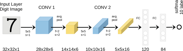
Legacy: Proved that learned features outperform hand-crafted features for vision tasks.

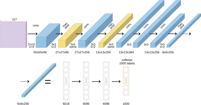
40. AlexNet (2012): The Deep Learning Revolution

• Won ImageNet competition by a massive margin (15.3% vs. 26.2% error)
• Key innovations:
  • ReLU activation (fast training, no vanishing gradients)
  • Dropout regularization (prevents overfitting)
  • GPU training (made deep networks practical)
  • 60 million parameters, 8 layers

41. Going Deeper: The Vanishing Gradient Problem

• After AlexNet: let’s just add more layers!
• Problem: Very deep networks (20+ layers) stop learning
• Gradients vanish as they flow through many layers
• Training loss plateaus — the network can’t be trained effectively

Deeper is not always better… unless you have a trick.

42. ResNet (2015): Skip Connections

The Residual Block:

\[\mathbf{y} = F(\mathbf{x}) + \mathbf{x}\]

• Instead of learning \(\mathbf{y} = F(\mathbf{x})\), learn the residual \(F(\mathbf{x}) = \mathbf{y} - \mathbf{x}\)
• The skip connection \(+ \mathbf{x}\) provides a gradient highway

graph LR
    X["x"] --> C1["Conv + ReLU"]
    C1 --> C2["Conv"]
    X -- "Skip<br>Connection" --> ADD["+ "]
    C2 --> ADD
    ADD --> R["ReLU"]
    R --> Y["y = F(x) + x"]

Note

ResNet enabled networks with 100+ layers. The 2015 ImageNet winner had 152 layers.

43. U-Net: Segmentation Architecture

• Designed for pixel-level classification (semantic segmentation)
• Encoder: Downsampling path (like a normal CNN)
• Decoder: Upsampling path (restores spatial resolution)
• Skip connections: Connect encoder to decoder at each level

graph TD
    I["Input Image"] --> E1["Encoder 1<br>(↓ 256)"]
    E1 --> E2["Encoder 2<br>(↓ 128)"]
    E2 --> B["Bottleneck<br>(64)"]
    B --> D2["Decoder 2<br>(↑ 128)"]
    D2 --> D1["Decoder 1<br>(↑ 256)"]
    D1 --> O["Output Mask"]
    E1 -. "skip" .-> D1
    E2 -. "skip" .-> D2

44. Section 5 Recap

Architecture	Year	Innovation	Use Case
LeNet	1995	Learned filters	Digit recognition
AlexNet	2012	ReLU, Dropout, GPU	Image classification
ResNet	2015	Skip connections	Very deep networks
U-Net	2015	Encoder-Decoder	Pixel segmentation

Section 6: Materials Science Case Studies

Slides 45–50

45. Case Study: Phase Segmentation in TEM

• Task: Segment crystalline Au nanoparticles from amorphous background
• Method: U-Net trained on labeled TEM frames
• Challenge: Limited labeled data, noisy images, beam damage

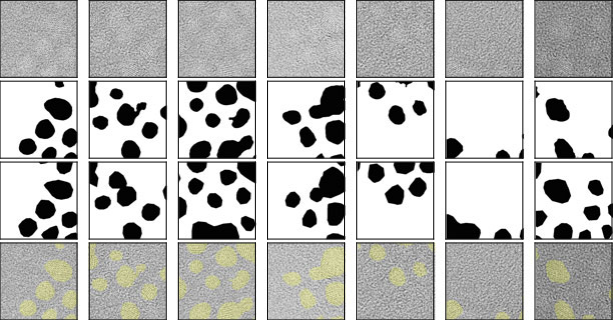
46. Case Study: Synthetic Training Data

• Problem: No labeled SEM grain microstructures available
• Solution: Generate synthetic grain structures using Voronoi tessellations
• Parameters: number of seeds, regularity, boundary thickness
• Result: Perfect labels for free — no expert annotation needed!

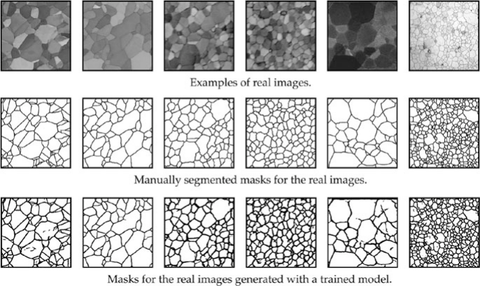
47. Case Study: Synthetic-to-Real Transfer

• Train only on Voronoi synthetic data
• Test on real polycrystalline SEM images
• Result: Nearly perfect grain boundary segmentation!

The synthetic data captured the topological truth of grain networks — the CNN learned grain boundary detection without ever seeing a real micrograph.

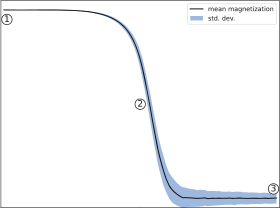
48. Case Study: Property Prediction from Microstructure

• Task: Classify Ising model microstructures by simulation temperature
• Input: 2D spin configurations (binary images)
• Method: CNN classifier trained on labeled configurations
• Result: CNN learns to detect the phase transition temperature from microstructure alone

49. Current Challenges

• Data scarcity: 50 labeled micrographs vs. 14M ImageNet images
• Domain gap: Natural images ≠ micrographs (contrast, texture, noise)
• 3D structures from 2D sections: Stereological sampling bias persists
• Interpretability: What does the CNN actually learn?

Next week: Strategies to overcome data scarcity — Transfer Learning, Augmentation, and Synthetic Data.

50. Unit 5 Summary & Next Steps

Key Takeaways:

1. Convolutions exploit spatial locality with shared weights
2. Weight sharing reduces parameters by orders of magnitude
3. Pooling provides downsampling and shift invariance
4. Feature hierarchies: edges → textures → morphologies → properties
5. U-Net is the standard for microstructure segmentation

Reading:

• Sandfeld (2024): Ch. 19 (CNNs) (Sandfeld et al. 2024)
• McClarren (2021): Ch. 6 (CNNs) (McClarren 2021)

Next Week: Unit 6 — Data Scarcity, Transfer Learning & Synthetic Data

References

McClarren, Ryan G. 2021. Machine Learning for Engineers: Using Data to Solve Problems for Physical Systems. Springer.

Sandfeld, Stefan et al. 2024. Materials Data Science. Springer.