flowchart LR
    subgraph "5-Fold Cross-Validation"
        direction TB
        F1["Fold 1: <b>Val</b> | Train | Train | Train | Train → e₁"]
        F2["Fold 2: Train | <b>Val</b> | Train | Train | Train → e₂"]
        F3["Fold 3: Train | Train | <b>Val</b> | Train | Train → e₃"]
        F4["Fold 4: Train | Train | Train | <b>Val</b> | Train → e₄"]
        F5["Fold 5: Train | Train | Train | Train | <b>Val</b> → e₅"]
    end
    F5 --> R["CV Score = (e₁+e₂+e₃+e₄+e₅) / 5"]
style R fill:#2d6a4f,stroke:#333,color:#fffMachine Learning in Materials Processing & Characterization
Unit 8: Generalization, Robustness, and Process Windows


03. Underfitting vs Overfitting
Underfitting
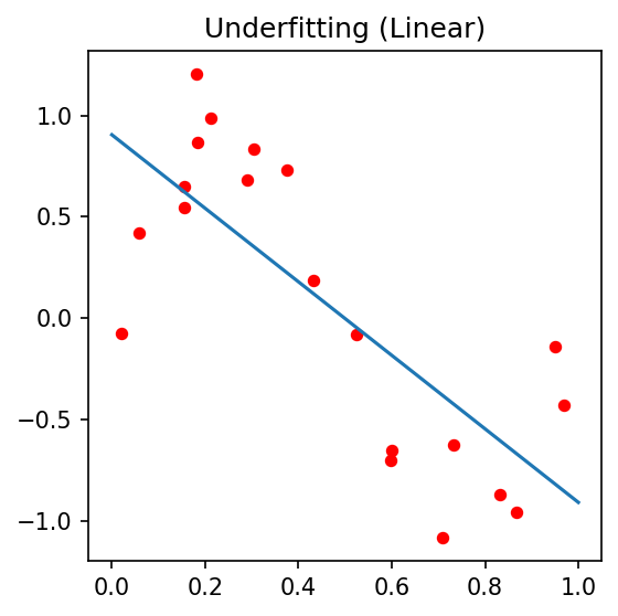
- Model is too simple
- High bias
- Misses the underlying pattern
- Example: Fitting a line to a nonlinear stress-strain curve
Good Fit
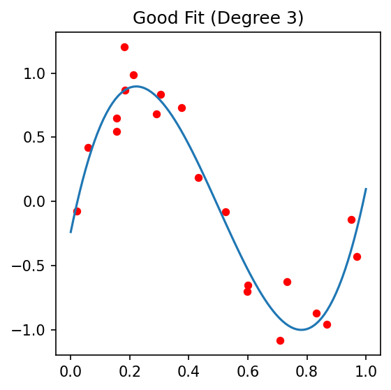
- Model captures the true relationship
- Balanced bias and variance
- Generalizes well to new data
Overfitting
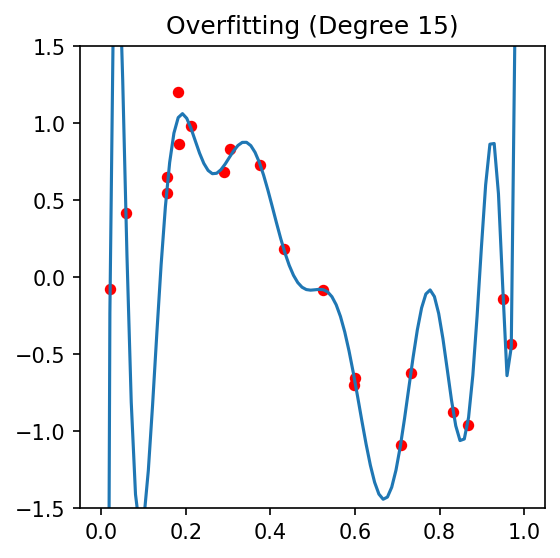
- Model is too complex
- High variance
- Memorizes noise
- Example: Degree-20 polynomial on 15 data points
04. The Bias-Variance Tradeoff
The Fundamental Decomposition
For a model \(\hat{f}(x)\) trained on data \(\mathcal{D}\), the expected prediction error at a point \(x\) is:
\[\text{EPE}(x) = \underbrace{\text{Bias}^2[\hat{f}(x)]}_{\text{systematic error}} + \underbrace{\text{Var}[\hat{f}(x)]}_{\text{sensitivity to training data}} + \underbrace{\sigma^2_\varepsilon}_{\text{irreducible noise}}\]
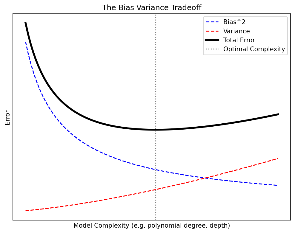
- As complexity increases: bias decreases, variance increases
- The optimal model sits at the minimum of total error
- The irreducible noise \(\sigma^2_\varepsilon\) sets a floor — no model can beat it
06. Polynomial Regression Example
Complexity vs Generalization (McClarren 2021)
Setup: \(n = 20\) noisy samples from \(f(x) = \sin(2\pi x)\)
| Polynomial Degree | Training MSE | Test MSE | Diagnosis |
|---|---|---|---|
| 1 | 0.42 | 0.45 | Underfitting (high bias) |
| 3 | 0.08 | 0.09 | Good fit |
| 9 | 0.001 | 0.35 | Overfitting (high variance) |
| 15 | \(\approx 0\) | 12.7 | Severe overfitting |

- Degree 3 has the best test error — not degree 15!
- Training error always decreases with complexity — but test error does not
19. L2 Regularization (Ridge Regression)
Shrinking Weights Toward Zero
\[J_\text{Ridge} = \sum_{i=1}^n (y_i - \hat{y}_i)^2 + \lambda \sum_{j=1}^p w_j^2 = \|\mathbf{y} - \mathbf{X}\mathbf{w}\|_2^2 + \lambda \|\mathbf{w}\|_2^2\]
Closed-form solution:
\[\hat{\mathbf{w}}_\text{Ridge} = (\mathbf{X}^\top \mathbf{X} + \lambda \mathbf{I})^{-1} \mathbf{X}^\top \mathbf{y}\]
Properties:
- Shrinks all weights proportionally toward zero
- Never sets weights exactly to zero — keeps all features
- Stabilizes ill-conditioned problems (adds \(\lambda\) to diagonal)
- Also called Tikhonov regularization in engineering/physics
Geometric interpretation:
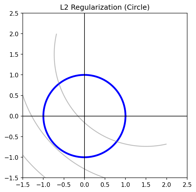
The L2 constraint defines a circle (sphere in higher dimensions). The regularized solution is where the loss contours first touch this circle.
20. L1 Regularization (Lasso)
Automatic Feature Selection Through Sparsity
\[J_\text{Lasso} = \|\mathbf{y} - \mathbf{X}\mathbf{w}\|_2^2 + \lambda \|\mathbf{w}\|_1 = \|\mathbf{y} - \mathbf{X}\mathbf{w}\|_2^2 + \lambda \sum_{j=1}^p |w_j|\]
Properties:
- Drives many weights to exactly zero
- Performs automatic feature selection
- Solution is sparse: only a subset of features are “active”
- No closed-form solution — requires iterative optimization
Geometric interpretation:
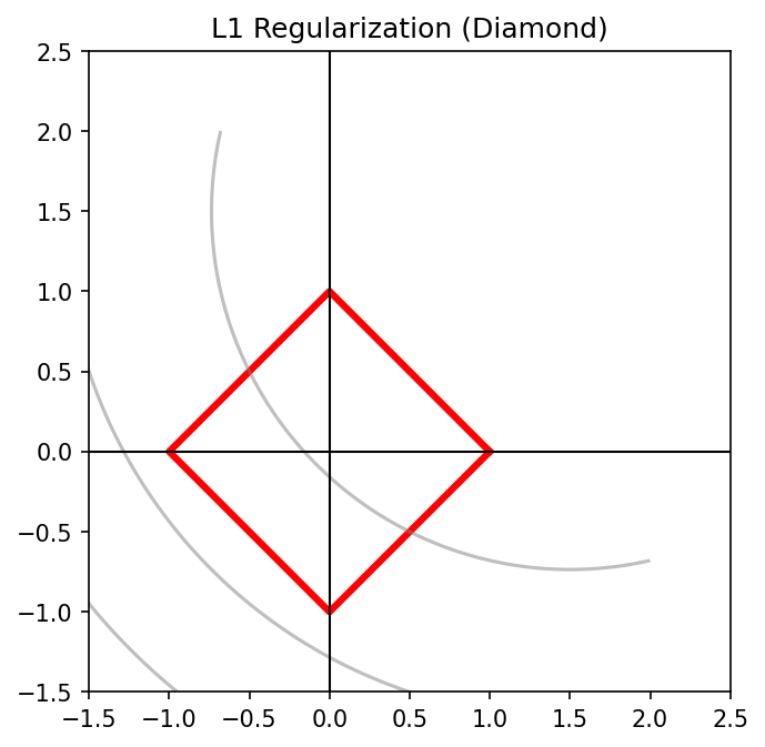
The L1 constraint defines a diamond (cross-polytope). The corners of the diamond lie on coordinate axes — so the loss contours often touch at a corner, setting one or more weights to exactly zero.
Materials application: With 100 candidate process parameters, Lasso can identify the 5-10 that truly matter — interpretable and physically meaningful.
21. L1 vs L2: A Visual Comparison
L2 (Ridge) — Circle
- Smooth constraint boundary
- Solution usually not on an axis
- All features retained with small weights
- Good for: correlated features, prediction
L1 (Lasso) — Diamond
- Pointy corners on axes
- Solution often at a corner → sparse
- Some features exactly zeroed out
- Good for: feature selection, interpretability
| Property | L2 (Ridge) | L1 (Lasso) |
|---|---|---|
| Weight behavior | Small but nonzero | Many exactly zero |
| Feature selection | No | Yes |
| Correlated features | Shares weight among correlated features | Picks one, zeros others |
| Computation | Closed-form | Iterative |
| Use case | Prediction with all features | Sparse, interpretable model |
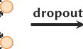
23. Dropout for Neural Networks
Randomly Disabling Neurons During Training (Goodfellow et al. 2016)
Idea: During each training step, randomly set each neuron’s output to zero with probability \(p\) (typically \(p = 0.2\) to \(0.5\)).
Why it works:
- Prevents co-adaptation — neurons cannot rely on specific other neurons
- Each training step trains a different “sub-network”
- Effectively an ensemble of \(2^n\) sub-networks (where \(n\) = number of neurons)
- At test time: use all neurons but scale outputs by \((1-p)\)
25. Early Stopping
The Simplest and Most Effective Regularizer
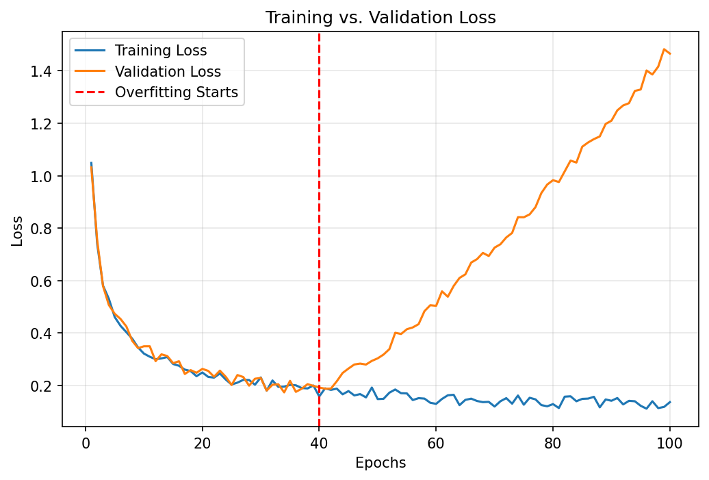
Principle:
- Training loss always decreases as training continues
- Validation loss decreases then increases (overfitting begins)
- Stop training at the minimum of validation loss
Implementation:
from sklearn.neural_network import MLPRegressor

# Or in PyTorch with a patience-based callback:
best_val_loss = float('inf')
patience, wait = 10, 0
for epoch in range(1000):
    train_loss = train_one_epoch(model, train_loader)
    val_loss = evaluate(model, val_loader)
    if val_loss < best_val_loss:
        best_val_loss = val_loss
        save_checkpoint(model)  # Save the best model
        wait = 0
    else:
        wait += 1
        if wait >= patience:
break # Stop training- Patience parameter: how many epochs to wait for improvement before stopping
- Acts as an implicit constraint on model complexity — limits effective number of parameters
33. Process Windows: Definition
The Safe Operating Region
A process window is the region in parameter space where:
- The target property meets its specification (e.g., density > 99.5%)
- The process is robust to expected noise levels
- The model prediction is confident (low uncertainty)
Formally:
\[\mathcal{W} = \left\{\mathbf{x} \in \mathbb{R}^p : \hat{f}(\mathbf{x}) \in [y_\text{min}, y_\text{max}] \;\wedge\; \|\nabla \hat{f}(\mathbf{x})\| < \tau \right\}\]
where \([y_\text{min}, y_\text{max}]\) is the specification range and \(\tau\) is the sensitivity threshold.
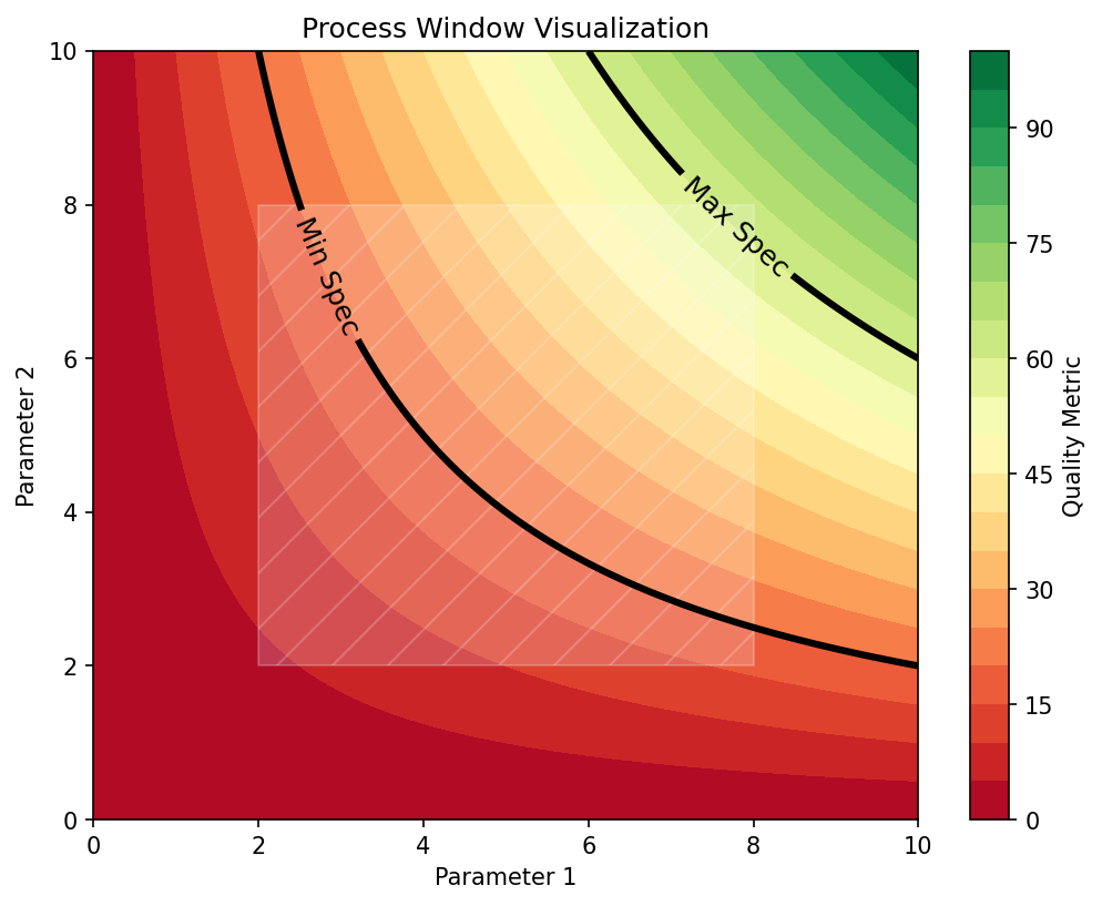
In additive manufacturing: The process window is the region in (Power, Speed) space that avoids both lack-of-fusion (insufficient melting) and keyhole (excessive vaporization) porosity.
35. Robust Optimization vs Peak Optimization
Choosing Where to Operate
Peak Optimization
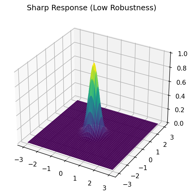
- Finds the maximum of the predicted property
- Operating point: \(\mathbf{x}^* = \arg\max_\mathbf{x} \hat{f}(\mathbf{x})\)
- Risk: Small deviations cause large quality drops
- Good for: laboratory research
Robust Optimization
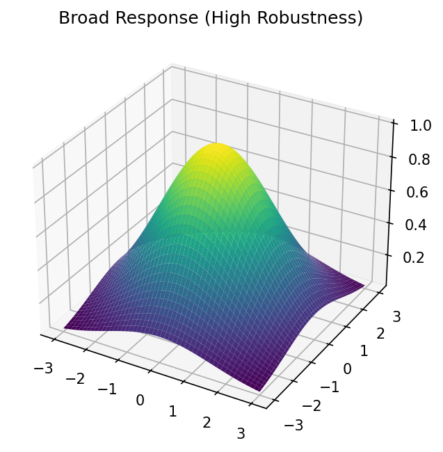
- Finds a plateau where the property is good AND stable
- \(\mathbf{x}^* = \arg\max_\mathbf{x}\left[\hat{f}(\mathbf{x}) - \kappa \|\nabla \hat{f}(\mathbf{x})\|\right]\)
- Benefit: Tolerates process noise
- Good for: production/manufacturing
The Engineering Tradeoff
In production, a 5% lower peak performance with 10× better robustness is almost always the right choice. A process that produces 98% density every time is more valuable than one that produces 99.5% density half the time and 95% density the other half.
36. Case Study: LPBF Keyhole Porosity Avoidance
Laser Powder Bed Fusion Process Window
Problem: In LPBF additive manufacturing, porosity arises from two mechanisms:
- Lack-of-fusion (too little energy): unmolten powder, large irregular pores
- Keyhole (too much energy): vapor depression traps gas, spherical pores
ML approach:
- Inputs: Laser power \(P\) [W], Scan speed \(v\) [mm/s], Layer thickness \(t\) [µm], Hatch spacing \(h\) [µm]
- Output: Relative density [%] or porosity classification
- Model: Random Forest trained on ~200 single-track experiments
Results:
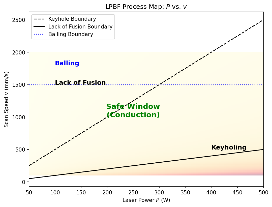
- The ML model identifies a band of safe parameters between two failure modes
- Sensitivity analysis reveals that \(P/v\) (linear energy density) is the dominant parameter
- The robust operating point is at the center of the safe band, not at the edge
40. Learning Curves: Diagnosis Tool
Identifying Bias vs Variance from Data
Learning curve: Plot training error and validation error as a function of training set size.
High Bias (Underfitting)
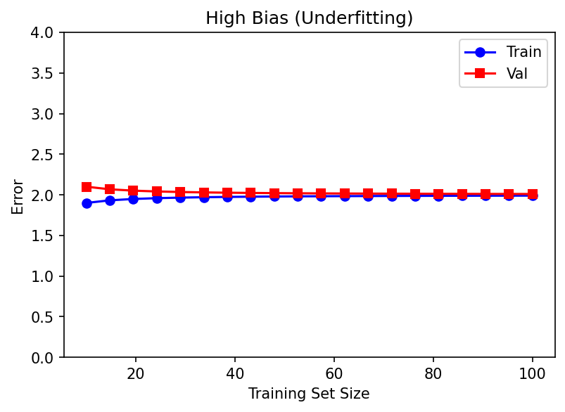
- Training error increases as data grows
- Validation error decreases but plateaus high
- Both converge to a large gap from target
- Fix: More complex model, better features
High Variance (Overfitting)
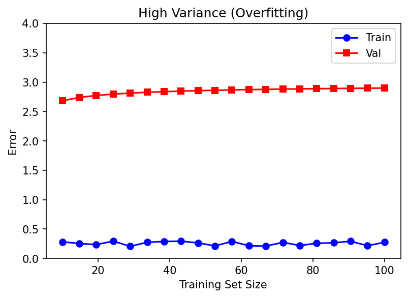
- Training error remains low
- Validation error remains high
- Large gap between training and validation
- Fix: More data, regularization, simpler model