Machine Learning in Materials Processing & Characterization
Unit 9: Inverse Problems and Process Maps

Prof. Dr. Philipp Pelz

FAU Erlangen-Nürnberg

01. Learning Outcomes

After this unit, you will be able to:

1. Distinguish forward from inverse problems and explain why inverse problems are ill-posed

2. Apply regularization strategies (Tikhonov, Bayesian priors) to stabilize inverse solutions

3. Construct process maps and identify safe operating windows for manufacturing

4. Formulate PINNs-based inverse problems to discover material parameters from data

5. Explain the SINDy algorithm and its use for discovering governing equations from data

Section 1: Forward / Inverse Duality

The Fundamental Asymmetry

02. Recap: Forward Modeling

Process → Structure → Properties

The forward problem is what we have been doing in previous units:

\[\mathbf{y} = f(\mathbf{x}) + \varepsilon\]

Given process parameters \(\mathbf{x}\), predict the resulting structure or properties \(\mathbf{y}\).

Examples:

Input \(\mathbf{x}\)	Model \(f\)	Output \(\mathbf{y}\)
Laser power, scan speed	Thermal simulation	Melt pool depth
Alloy composition	CALPHAD	Phase fractions
Annealing time, temperature	Diffusion model	Grain size

• Forward problems are typically well-posed: the output is uniquely determined by the input
• Physics gives us the direction of causality: cause \(\rightarrow\) effect

03. What Is an Inverse Problem?

Structure → Process

The inverse problem reverses the arrow:

\[\mathbf{x} = f^{-1}(\mathbf{y})\]

Given the desired output \(\mathbf{y}^*\), find the input \(\mathbf{x}^*\) that produces it.

The question engineers actually ask:

• “I need a part with \(< 0.1\%\) porosity — what laser parameters should I use?”
• “I want a grain size of \(10\,\mu\text{m}\) — what annealing schedule gives me that?”
• “I need yield strength \(> 800\,\text{MPa}\) — what alloy composition and heat treatment?”

flowchart LR
    A["Desired Properties<br>y*"] -->|"Inverse Problem<br>x = f⁻¹(y)"| B["Required Process<br>x*"]
    B -->|"Forward Problem<br>y = f(x)"| C["Achieved Properties<br>y"]
    C -->|"Compare"| A
    style A fill:#e74c3c,color:#fff
    style B fill:#2ecc71,color:#fff
    style C fill:#3498db,color:#fff

04. The Challenge: Non-Uniqueness

Many Inputs Can Produce the Same Output

If the forward map \(f\) is many-to-one, then \(f^{-1}\) is one-to-many:

\[f(\mathbf{x}_1) = f(\mathbf{x}_2) = \ldots = f(\mathbf{x}_k) = \mathbf{y}^*\]

Materials example:

A grain size of \(d = 10\,\mu\text{m}\) can be achieved by:

• High temperature, short time: \((T_1 = 1100°\text{C},\; t_1 = 5\,\text{min})\)
• Moderate temperature, medium time: \((T_2 = 900°\text{C},\; t_2 = 60\,\text{min})\)
• Low temperature, long time: \((T_3 = 750°\text{C},\; t_3 = 480\,\text{min})\)

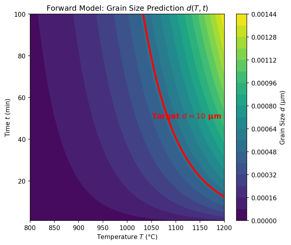
• The forward problem has one answer; the inverse has infinitely many
• Which solution should we choose? Physics alone does not decide — we need additional criteria

05. Why Standard NNs Fail for Inverse Problems

The Averaging Problem

Train a standard neural network to map \(\mathbf{y} \rightarrow \mathbf{x}\) using MSE loss:

\[\mathcal{L} = \frac{1}{N}\sum_{i=1}^{N} \|\mathbf{x}_i - \hat{\mathbf{x}}(\mathbf{y}_i)\|^2\]

If multiple valid solutions \(\{\mathbf{x}_1, \mathbf{x}_2, \mathbf{x}_3\}\) exist for the same \(\mathbf{y}^*\):

\[\hat{\mathbf{x}}_\text{NN} \approx \frac{1}{k}\sum_{j=1}^{k}\mathbf{x}_j \quad \text{(the mean of valid solutions)}\]

The mean of valid solutions is often not itself a valid solution!

The Averaging Trap

A standard neural network trained with MSE loss on an inverse problem will predict the average of all valid solutions. This average may lie in a region of parameter space that produces defective parts — it is a physically meaningless compromise.

Section 2: Ill-Posedness & Regularization

Taming Unstable Solutions

06. Hadamard’s Definition of Well-Posedness

Three Conditions (Jacques Hadamard, 1902)

A problem is well-posed if and only if all three conditions hold:

1. Existence: A solution exists for every admissible input

2. Uniqueness: The solution is unique

3. Stability: The solution depends continuously on the data — small changes in input produce small changes in output

A problem that violates any of these conditions is called ill-posed.

Condition	Forward Problem	Inverse Problem
Existence	Usually yes	May fail (no process gives exactly \(\mathbf{y}^*\))
Uniqueness	Usually yes	Often fails (many-to-one forward map)
Stability	Usually yes	Often fails (noise amplification)

07. When Problems Are Ill-Posed

The Butterfly Effect in Inversion

Stability violation — noise amplification:

If the forward model maps a large range of inputs to a narrow range of outputs, then the inverse must map a narrow range of outputs back to a large range of inputs.

\[\text{Forward: } \Delta x = 100 \;\rightarrow\; \Delta y = 1\] \[\text{Inverse: } \Delta y = 1 \;\rightarrow\; \Delta x = 100\]

A \(1\%\) measurement error in \(y\) causes a \(100\%\) error in the inferred \(x\)!

Materials example:

• Measuring porosity with \(\pm 0.05\%\) accuracy
• The inverse map amplifies this to \(\pm 50\,\text{W}\) uncertainty in laser power
• This spans the entire range between “good” and “keyholing” regimes

08. Think About This…

The Tomography Puzzle

You have an X-ray CT scanner and take projection images of a metal part from 180 angles.

The forward problem is straightforward:

\[p_\theta(s) = \int_{\text{ray}} \mu(x, y)\, dl\]

Each projection is a line integral of the attenuation coefficient \(\mu(x, y)\).

Question 1: Is the inverse problem (reconstructing \(\mu(x, y)\) from projections) well-posed?

\(\rightarrow\) It depends! With infinite noiseless projections, it is well-posed (Radon transform is invertible). With finitely many noisy projections, it is ill-posed — many images are consistent with the data.

Question 2: What happens if you reduce from 180 projections to 10?

\(\rightarrow\) The problem becomes severely ill-posed. The null space of the measurement operator grows — there are many structures that produce the same 10 projections. You need strong priors (sparsity, smoothness, physics) to regularize.

09. Regularization: Prior Knowledge as a Constraint

Turning Ill-Posed into Well-Posed

Core idea: We cannot solve the inverse problem from data alone — we need to add prior knowledge about what a “good” solution looks like.

\[\hat{\mathbf{x}} = \arg\min_{\mathbf{x}} \underbrace{\|f(\mathbf{x}) - \mathbf{y}_\text{obs}\|^2}_{\text{data fidelity}} + \lambda \underbrace{R(\mathbf{x})}_{\text{regularization}}\]

Regularizer \(R(\mathbf{x})\)	Prior assumption	Effect
\(\|\mathbf{x}\|_2^2\) (L2 / Ridge)	Parameters are small	Smooth solutions, shrinks all parameters
\(\|\mathbf{x}\|_1\) (L1 / LASSO)	Solution is sparse	Feature selection, sets parameters to zero
\(\|\nabla \mathbf{x}\|_2^2\)	Solution is smooth	Suppresses oscillations
Total Variation \(\|\nabla \mathbf{x}\|_1\)	Piecewise constant	Preserves sharp edges

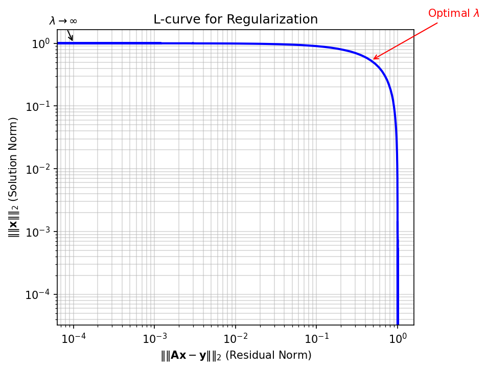
• \(\lambda\) controls the tradeoff between fitting data and satisfying the prior
• Too small \(\lambda\): noise dominates (overfitting to noisy measurements)
• Too large \(\lambda\): prior dominates (underfitting the data)

10. Physics as a Regularizer

The Most Powerful Prior

Instead of generic mathematical penalties, we can use physical laws as regularizers:

\[\hat{\mathbf{x}} = \arg\min_{\mathbf{x}} \|\mathbf{y}_\text{obs} - f(\mathbf{x})\|^2 + \lambda_\text{PDE} \underbrace{\left\|\mathcal{N}[\mathbf{u}(\mathbf{x})]\right\|^2}_{\text{PDE residual}} + \lambda_\text{BC} \underbrace{\left\|\mathcal{B}[\mathbf{u}(\mathbf{x})]\right\|^2}_{\text{boundary conditions}}\]

Physical constraints in materials science:

• Conservation of mass, momentum, energy
• Thermodynamic equilibrium (Gibbs energy minimization)
• Constitutive laws (stress-strain relations)
• Symmetry constraints (crystal symmetries)

Advantage over L1/L2:

• Physics-based regularizers encode domain knowledge, not just mathematical smoothness
• They constrain the solution to the physically realizable manifold
• They dramatically reduce the space of admissible solutions

11. Tikhonov Regularization

The Classical Approach

Tikhonov regularization (also called Ridge regression in ML) adds an L2 penalty:

\[\hat{\mathbf{x}} = \arg\min_{\mathbf{x}} \|\mathbf{A}\mathbf{x} - \mathbf{y}\|_2^2 + \lambda \|\mathbf{L}\mathbf{x}\|_2^2\]

For the linear case \(\mathbf{y} = \mathbf{A}\mathbf{x}\), the solution is:

\[\hat{\mathbf{x}}_\lambda = (\mathbf{A}^T\mathbf{A} + \lambda \mathbf{L}^T\mathbf{L})^{-1}\mathbf{A}^T\mathbf{y}\]

Effect on the singular values:

• Without regularization: \(\hat{x}_i = \frac{\sigma_i}{\sigma_i^2} (\mathbf{u}_i^T\mathbf{y})\) — small singular values \(\sigma_i\) cause blow-up
• With regularization: \(\hat{x}_i = \frac{\sigma_i}{\sigma_i^2 + \lambda} (\mathbf{u}_i^T\mathbf{y})\) — the \(\lambda\) term damps small singular values

12. Bayesian View of Inverse Problems

From Point Estimates to Posterior Distributions

Instead of finding a single “best” \(\mathbf{x}\), compute the posterior distribution:

\[p(\mathbf{x} \mid \mathbf{y}) = \frac{p(\mathbf{y} \mid \mathbf{x})\, p(\mathbf{x})}{p(\mathbf{y})}\]

Bayesian Term	Inverse Problem Meaning
\(p(\mathbf{x} \mid \mathbf{y})\) — Posterior	Probability of parameters given observed data
\(p(\mathbf{y} \mid \mathbf{x})\) — Likelihood	How well the forward model fits the data
\(p(\mathbf{x})\) — Prior	Our regularization / domain knowledge
\(p(\mathbf{y})\) — Evidence	Normalization constant

Connection to regularization:

• Gaussian prior \(p(\mathbf{x}) \propto \exp(-\frac{\lambda}{2}\|\mathbf{x}\|^2)\) \(\;\Leftrightarrow\;\) L2 (Tikhonov) regularization
• Laplace prior \(p(\mathbf{x}) \propto \exp(-\lambda\|\mathbf{x}\|_1)\) \(\;\Leftrightarrow\;\) L1 (LASSO) regularization
• The MAP estimate \(\hat{\mathbf{x}}_\text{MAP} = \arg\max_\mathbf{x}\, p(\mathbf{x} \mid \mathbf{y})\) recovers the regularized solution

Why Go Bayesian?

The posterior distribution gives us not just a point estimate but uncertainty quantification: we know which process parameters are well-constrained by the data and which are uncertain. This is essential for risk-aware manufacturing.

Section 3: Process Maps & Corridors

Navigating the Parameter Space

13. What Is a Process Map?

Visualizing the Feasible Region (Neuer et al. 2024)

A process map is a visualization of the parameter space that classifies regions by outcome quality:

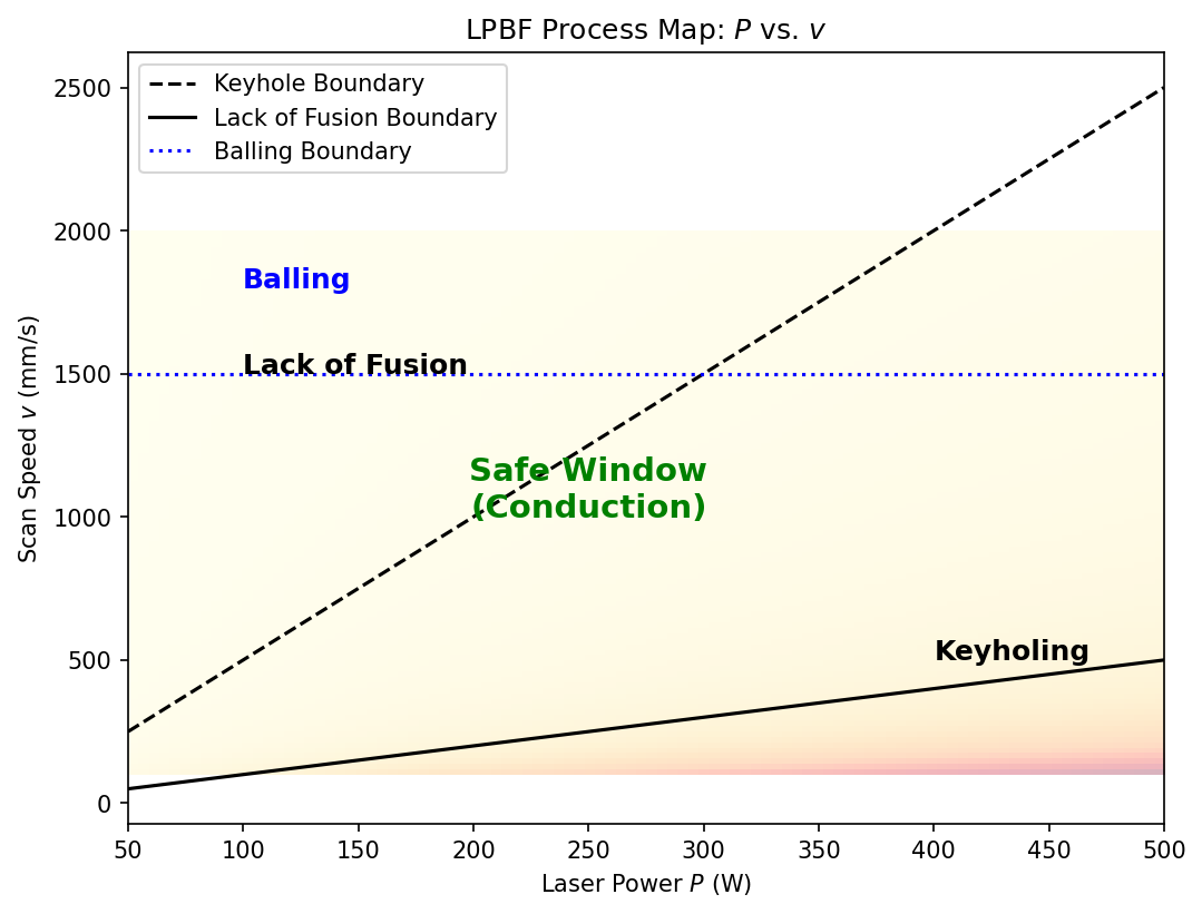
• Axes: Key process parameters (e.g., laser power \(P\), scan speed \(v\))
• Regions: Classified by dominant defect mechanism or quality metric
• Boundaries: Critical transitions between regimes

The engineering goal: Find the region in parameter space where all quality criteria are simultaneously satisfied — the safe operating window.

14. Defining the Safe Operating Window

Defect Mechanisms as Constraints

Each defect mechanism defines a constraint boundary in parameter space:

Defect	Mechanism	Boundary condition
Keyholing	Vapor depression collapse	\(E_v > E_\text{keyhole}^*\) (energy density too high)
Lack of fusion	Insufficient melting	\(E_v < E_\text{fusion}^*\) (energy density too low)
Balling	Rayleigh instability	\(v > v_\text{ball}^*(P)\) (speed too high for given power)
Cracking	Thermal stress	\(\dot{T} > \dot{T}_\text{crack}^*\) (cooling rate too high)

The safe operating window is the intersection:

\[\Omega_\text{safe} = \{\mathbf{x} : E_v(\mathbf{x}) \in [E_\text{fusion}^*, E_\text{keyhole}^*] \;\wedge\; v < v_\text{ball}^*(P) \;\wedge\; \dot{T} < \dot{T}_\text{crack}^*\}\]

• In LPBF, the volumetric energy density is often used: \(E_v = \frac{P}{v \cdot h \cdot t}\)
• The safe window may be narrow — leaving little room for process variation

15. Process Corridors

Drift Over Time (Neuer et al. 2024)

A process corridor extends the static process map to account for temporal drift:

• Equipment degradation (laser power drift, optics contamination)
• Raw material variation (powder reuse, batch-to-batch variability)
• Environmental changes (humidity, ambient temperature)

The corridor concept:

• The nominal operating point is the center of the safe window
• The corridor is the trajectory of the actual operating point over time
• If the corridor exits the safe window, defects occur
• Monitoring the corridor enables predictive maintenance and adaptive process control

16. Multi-Dimensional Feasibility Regions

Beyond 2D Maps

Real manufacturing processes have many more than 2 parameters:

LPBF example — at least 8 key parameters:

Parameter	Typical Range
Laser power \(P\)	100 – 500 W
Scan speed \(v\)	200 – 2000 mm/s
Hatch spacing \(h\)	50 – 150 μm
Layer thickness \(t\)	20 – 100 μm
Spot diameter \(d\)	50 – 200 μm
Preheat temperature \(T_0\)	25 – 500 °C
Scan strategy	Stripe, island, meander
Gas flow rate	1 – 10 m/s

• The feasible region is a high-dimensional manifold that cannot be visualized directly
• 2D process maps are projections — they can hide important interactions
• ML enables navigation of the full-dimensional space

17. ML for Mapping Defect Boundaries

Classification Approach

Idea: Train a classifier to predict defect type from process parameters:

\[\hat{c}(\mathbf{x}) = \text{Classifier}(P, v, h, t, d, T_0, \ldots)\]

where \(c \in \{\text{dense}, \text{keyhole}, \text{LOF}, \text{balling}, \text{cracking}\}\)

Common approaches:

• Random Forests: Handle mixed parameter types, provide feature importance
• SVM: Good boundaries with limited data, kernel methods for non-linear boundaries
• Neural Networks: Flexible boundaries, but need more data
• Gaussian Processes: Provide uncertainty on boundary location

flowchart LR
    A["Experimental Database<br>(parameters, outcomes)"] --> B["Train Classifier<br>(RF, SVM, GP, NN)"]
    B --> C["Decision Boundaries<br>in Parameter Space"]
    C --> D["Process Map<br>with Confidence"]
    D --> E["Safe Operating Window<br>+ Uncertainty"]
    style A fill:#3498db,color:#fff
    style B fill:#9b59b6,color:#fff
    style C fill:#e67e22,color:#fff
    style D fill:#2ecc71,color:#fff
    style E fill:#1abc9c,color:#fff

18. Sensitivity Analysis on the Process Map

Which Parameters Matter Most?

Sensitivity analysis identifies which process parameters have the strongest influence on quality:

Local sensitivity (gradient-based):

\[S_i = \frac{\partial \hat{y}}{\partial x_i}\bigg|_{\mathbf{x}_0}\]

How much does the output change when parameter \(i\) is perturbed?

Global sensitivity (Sobol indices):

\[S_i = \frac{\text{Var}[\mathbb{E}[\hat{y} \mid x_i]]}{\text{Var}[\hat{y}]}\]

What fraction of the total output variance is attributable to parameter \(i\)?

Materials insight: If the safe operating window is narrow along parameter \(x_i\) but wide along \(x_j\):

• \(x_i\) requires tight control (high sensitivity)
• \(x_j\) can tolerate more variation (low sensitivity)
• Focus monitoring and control efforts on the high-sensitivity parameters

19. Summary: Process Maps

Key concepts:

• Process maps visualize feasibility regions in parameter space, bounded by defect mechanisms

• The safe operating window is the intersection of all quality constraints

• Process corridors capture temporal drift of the operating point

• ML classifiers can learn defect boundaries from experimental data

• Sensitivity analysis identifies which parameters require tightest control

• Finding the optimal operating point within the safe window is an inverse problem

Section 4: Parameter Discovery with PINNs

From Data to Physics

20. PINNs for Inverse Problems

Recap: The PINN Framework

Recall from Unit 7: A Physics-Informed Neural Network represents the solution \(u(x, t)\) as a neural network and trains it by minimizing:

\[\mathcal{L} = \underbrace{\mathcal{L}_\text{data}}_{\text{match observations}} + \underbrace{\lambda_\text{PDE}\, \mathcal{L}_\text{PDE}}_{\text{satisfy physics}} + \underbrace{\lambda_\text{BC}\, \mathcal{L}_\text{BC}}_{\text{boundary conditions}}\]

Forward PINN: All parameters of the PDE are known. The network learns \(u(x,t)\).

Inverse PINN: Some parameters of the PDE are unknown. The network learns \(u(x,t)\) and the unknown parameters simultaneously.

Key insight: Unknown physical parameters (diffusivity, conductivity, viscosity) become trainable parameters of the optimization, alongside the network weights.

21. Case Study: Discovering Thermal Diffusivity

The Heat Equation with Unknown \(\alpha\) (McClarren 2021)

The heat equation:

\[\frac{\partial T}{\partial t} = \alpha \nabla^2 T\]

where \(\alpha\) is the thermal diffusivity — unknown.

Data: Temperature measurements \(T_\text{obs}(x_i, t_j)\) at scattered sensor locations.

Inverse PINN setup:

1. Network: \(\hat{T}(x, t; \boldsymbol{\theta})\) approximates the temperature field
2. Unknown: \(\alpha\) is a trainable scalar parameter
3. Minimize:

\[\mathcal{L} = \frac{1}{N_d}\sum_{i=1}^{N_d}\left(\hat{T}(x_i, t_i) - T_\text{obs}^i\right)^2 + \frac{\lambda}{N_c}\sum_{j=1}^{N_c}\left(\frac{\partial \hat{T}}{\partial t} - \alpha \nabla^2 \hat{T}\right)^2_{\!(x_j, t_j)}\]

22. The Inverse Loss Function

Anatomy of \(\mathcal{J} = \mathcal{J}_\text{data} + \mathcal{J}_\text{PDE}\)

flowchart TB
    subgraph Inputs
        X["Spatial coordinates x"]
        T["Time t"]
    end
    subgraph Network["Neural Network NN(x,t; θ)"]
        H1["Hidden layers"]
    end
    subgraph Outputs
        U["Predicted field û"]
    end
    subgraph AutoDiff["Automatic Differentiation"]
        DU["∂û/∂t, ∇²û"]
    end
    subgraph Loss["Total Loss"]
        LD["J_data = ||û - u_obs||²"]
        LP["J_PDE = ||∂û/∂t - α∇²û||²"]
    end
    subgraph Params["Trainable Parameters"]
        TH["Network weights θ"]
        AL["Unknown physics α"]
    end
    X --> Network
    T --> Network
    Network --> U
    U --> AutoDiff
    U --> LD
    AutoDiff --> LP
    AL --> LP
    LD --> |"Backprop"| TH
    LP --> |"Backprop"| TH
    LP --> |"Backprop"| AL
    style AL fill:#e74c3c,color:#fff
    style LD fill:#3498db,color:#fff
    style LP fill:#2ecc71,color:#fff

• Gradients of \(\mathcal{L}\) w.r.t. \(\alpha\) flow through the PDE residual via automatic differentiation
• The optimizer simultaneously updates \(\boldsymbol{\theta}\) (network weights) and \(\alpha\) (physics)

23. Why PINNs Beat Curve Fitting

Advantages of the Physics-Informed Approach

Traditional approach — least-squares curve fitting:

1. Assume a parametric form: \(T(x, t; \alpha) = T_0 + \Delta T\, \text{erfc}\!\left(\frac{x}{2\sqrt{\alpha t}}\right)\)
2. Fit \(\alpha\) by minimizing \(\sum_i (T_\text{model}^i - T_\text{obs}^i)^2\)

Problems with curve fitting:

• Requires an analytical solution — only available for simple geometries and BCs
• Cannot handle complex domains, nonlinear PDEs, or coupled physics
• Sensitive to noise — no regularization from the PDE structure

PINN advantages:

• Works with any PDE — no analytical solution needed
• Handles arbitrary geometries and boundary conditions
• The PDE itself acts as a regularizer, denoising the observations
• Can discover spatially varying parameters: \(\alpha(x)\) instead of a single scalar
• Naturally extends to multi-physics problems

24. Discovering Variable Parameters: \(D(T)\)

Beyond Scalar Constants

Many material properties depend on temperature or composition:

\[\frac{\partial c}{\partial t} = \nabla \cdot [D(T)\, \nabla c]\]

where \(D(T)\) is the temperature-dependent diffusivity — unknown functional form.

PINN approach:

• Represent \(D(T)\) as a second neural network: \(\hat{D}(T; \boldsymbol{\phi})\)
• Train simultaneously:
  • \(\hat{c}(x, t; \boldsymbol{\theta})\) — concentration field
  • \(\hat{D}(T; \boldsymbol{\phi})\) — diffusivity function

\[\mathcal{L} = \underbrace{\sum_i (c_\text{obs}^i - \hat{c}^i)^2}_{\text{data}} + \lambda \underbrace{\sum_j \left(\frac{\partial \hat{c}}{\partial t} - \nabla \cdot [\hat{D}(\hat{T}) \nabla \hat{c}]\right)^2_j}_{\text{PDE}} + \mu \underbrace{\sum_k \left(\frac{d\hat{D}}{dT}\right)^2_k}_{\text{smoothness prior on } D}\]

Result: We discover the full functional relationship \(D(T)\) from data — not just a single number!

25. Example: Melt Pool Shapes to Thermal Conductivity

Inverse Problem in Additive Manufacturing

Scenario: You have cross-sectional images of melt pool shapes from LPBF experiments at various process parameters.

Forward model: Steady-state heat equation with convection:

\[\rho c_p (\mathbf{v} \cdot \nabla T) = \nabla \cdot [k(T)\, \nabla T] + Q_\text{laser}\]

Known: Laser power \(Q_\text{laser}\), scan speed \(\mathbf{v}\), melt pool boundary (solidus isotherm location)

Unknown: Temperature-dependent thermal conductivity \(k(T)\)

Inverse PINN:

• The melt pool boundary provides data: \(\hat{T}(x_\text{boundary}) = T_\text{solidus}\)
• The PDE provides physics: heat equation residual
• The network learns \(k(T)\) that produces the observed melt pool shapes

26. Accuracy and Convergence

How Well Do Inverse PINNs Work?

Typical accuracy for parameter discovery:

Problem	Unknown	Relative Error	Data Points
1D Heat equation	\(\alpha\) (scalar)	\(< 1\%\)	100
2D Diffusion	\(D\) (scalar)	\(1\text{–}3\%\)	500
Navier-Stokes	\(\nu\) (viscosity)	\(2\text{–}5\%\)	1000
Variable \(D(T)\)	\(D(T)\) (function)	\(5\text{–}10\%\)	2000

Convergence challenges:

• Inverse PINNs are harder to train than forward PINNs — the loss landscape is more complex
• Multiple local minima may correspond to different physical parameters
• The balance \(\lambda\) between data and PDE loss is critical
• Strategies: Learning rate scheduling, curriculum training (start with data, add PDE gradually), multi-fidelity approaches

Practical Tip

Start the inverse PINN training with a good initial guess for the unknown parameter. If \(\alpha_\text{true} \approx 10^{-5}\), initializing at \(\alpha_0 = 10^{-7}\) may converge to a wrong local minimum. Use rough estimates from literature or dimensional analysis.

27. Traditional Inverse Methods vs PINNs

A Fair Comparison

Criterion	Traditional (Adjoint/FEM)	PINNs
Mesh requirement	Yes (FEM mesh)	No (meshfree)
Analytical solution	Sometimes needed	Never needed
Complex geometry	Challenging meshing	Easy (point sampling)
Nonlinear PDEs	Iterative, expensive	Natural (backprop)
Spatially varying parameters	Parameterization needed	Network approximation
Uncertainty quantification	Adjoint-based	Ensemble/Bayesian NN
Computational cost	One FEM solve per iteration	One training run
Maturity	Decades of development	Rapidly evolving
Industrial adoption	Widespread	Early stage

Bottom line: PINNs are not always better — but they offer unique advantages for complex, multi-physics, data-scarce problems where meshing or analytical solutions are impractical.

28. Inverse Problems in Tomography

ML-Enhanced Reconstruction

Classical reconstruction:

\[\hat{\mu}(x, y) = \text{FBP}[p_\theta(s)] \quad \text{(Filtered Backprojection)}\]

Works well with many projections, but fails with limited/noisy data.

ML inverse approaches:

1. Learned post-processing: FBP → CNN denoiser
2. Learned iterative reconstruction: Unrolled optimization with learned regularizers
3. Direct inversion: Train network to map sinograms to images
4. Physics-informed: PDE-constrained reconstruction (e.g., beam hardening model)

Why it matters for materials:

• In-situ tomography during solidification: few projections, fast acquisition
• Electron tomography: limited tilt range (missing wedge problem)
• Neutron tomography: low SNR, need strong regularization

29. Multi-Physics Inversion

Coupling Multiple Governing Equations

Real manufacturing involves coupled physics:

\[\text{Thermal} \longleftrightarrow \text{Mechanical} \longleftrightarrow \text{Microstructural} \longleftrightarrow \text{Fluid}\]

Multi-physics inverse PINN:

\[\mathcal{L} = \mathcal{L}_\text{data} + \lambda_1 \mathcal{L}_\text{heat} + \lambda_2 \mathcal{L}_\text{Navier-Stokes} + \lambda_3 \mathcal{L}_\text{phase-field} + \lambda_4 \mathcal{L}_\text{mechanics}\]

Example — LPBF multi-physics inversion:

• Observe: Surface temperature (thermal camera) + melt pool shape (high-speed video)
• Discover: Absorptivity \(\eta\), Marangoni coefficient \(\partial\gamma/\partial T\), mushy zone constant \(A_\text{mush}\)
• Constrained by: Heat equation + Navier-Stokes + Stefan condition

Challenge: Balancing loss terms \(\lambda_1, \ldots, \lambda_4\) becomes critical — active research area (adaptive weighting, gradient normalization)

30. From Data to Digital Twin

The Inverse Problem Perspective

A digital twin is a continuously updated computational model of a physical system:

1. Initialization: Solve inverse problem to calibrate model parameters from initial data
2. Prediction: Run forward model to predict future behavior
3. Update: As new data arrives, solve inverse problem again to update parameters
4. Control: Use updated model to optimize process parameters (another inverse problem!)

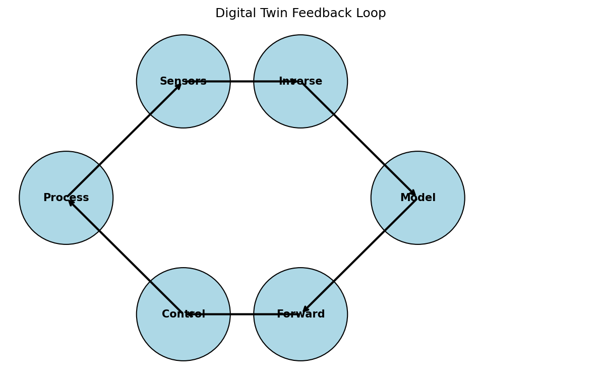
The inverse problem is at the heart of every digital twin:

• Without inversion, the model is a static simulation — not a twin
• The “twin” aspect comes from continuous calibration against real-world data

31. Summary: PINN Inversion

Key concepts:

• PINNs solve inverse problems by making unknown physical parameters trainable

• They can discover scalar constants (\(\alpha\), \(k\), \(\nu\)) or functional relationships (\(D(T)\), \(k(T)\))

• The PDE acts as a physics-based regularizer, stabilizing the ill-posed inverse problem

• PINNs excel at meshfree, multi-physics problems with scattered data

• Challenges include training stability, loss balancing, and convergence to local minima

• The digital twin concept relies on continuous inverse problem solving for model calibration

Section 5: Equation Discovery — SINDy

Discovering Governing Equations from Data

32. Symbolic Regression: The Idea

From Data to Equations

Standard regression: Fit parameters of a known model

\[y = a_0 + a_1 x + a_2 x^2 \quad \text{(we chose the form, fit the } a_i\text{)}\]

Symbolic regression: Discover both the form and the parameters

\[y = ??? \quad \text{(find the equation itself from data)}\]

The dream:

Input Data	Discovered Equation
Planetary orbits	\(F = \frac{Gm_1 m_2}{r^2}\)
Pendulum motion	\(\ddot{\theta} = -\frac{g}{l}\sin\theta\)
Cooling curves	\(\frac{dT}{dt} = -h(T - T_\infty)\)
Stress-strain data	\(\sigma = K\varepsilon^n\)

Challenge: The space of possible equations is combinatorially vast — brute force search is infeasible

33. SINDy: Sparse Identification of Nonlinear Dynamics

The Key Insight (Brunton et al. 2016) (McClarren 2021)

Observation: Most physical laws involve only a few terms from a large space of possible terms.

\[\frac{d\mathbf{x}}{dt} = f(\mathbf{x}) = \boldsymbol{\Theta}(\mathbf{x})\, \boldsymbol{\xi}\]

where:

• \(\mathbf{x}(t)\) — measured state variables (e.g., position, temperature, concentration)
• \(\dot{\mathbf{x}}\) — time derivatives (estimated from data)
• \(\boldsymbol{\Theta}(\mathbf{x})\) — library of candidate functions (many columns)
• \(\boldsymbol{\xi}\) — sparse coefficient vector (mostly zeros!)

flowchart LR
    A["Measurement Data<br>x(t)"] --> B["Compute Derivatives<br>ẋ(t)"]
    B --> C["Build Library<br>Θ(x) = [1, x, x², sin(x), ...]"]
    C --> D["Sparse Regression<br>ẋ = Θξ, minimize ||ξ||₁"]
    D --> E["Discovered Equation<br>ẋ = -0.5x + 0.1x³"]
    style A fill:#3498db,color:#fff
    style B fill:#9b59b6,color:#fff
    style C fill:#e67e22,color:#fff
    style D fill:#e74c3c,color:#fff
    style E fill:#2ecc71,color:#fff

34. The Function Library \(\boldsymbol{\Theta}\)

Building the Dictionary of Candidates

For state variables \(\mathbf{x} = [x_1, x_2]\), a typical library includes:

\[\boldsymbol{\Theta}(\mathbf{x}) = \begin{bmatrix} 1 & x_1 & x_2 & x_1^2 & x_1 x_2 & x_2^2 & x_1^3 & \ldots & \sin(x_1) & \cos(x_1) & \ldots \end{bmatrix}\]

Design choices:

Choice	Tradeoff
Polynomials up to degree \(d\)	Higher \(d\) → more expressive but more columns → harder sparsity
Trigonometric functions	Include if oscillatory behavior expected
Cross-terms \(x_i x_j\)	Capture interactions between state variables
Domain-specific terms	\(e^{-E_a/RT}\) for Arrhenius, \(x(1-x)\) for logistic growth

The library should be:

• Rich enough to contain the true terms
• Not too large — more columns means more spurious correlations
• Informed by domain knowledge — include physically motivated terms

35. Sparse Regression: LASSO

Finding the Sparse Coefficients

The optimization problem:

\[\hat{\boldsymbol{\xi}} = \arg\min_{\boldsymbol{\xi}} \|\dot{\mathbf{X}} - \boldsymbol{\Theta}(\mathbf{X})\boldsymbol{\xi}\|_2^2 + \lambda \|\boldsymbol{\xi}\|_1\]

• The L1 penalty \(\|\boldsymbol{\xi}\|_1\) promotes sparsity — drives small coefficients to exactly zero
• \(\lambda\) controls the sparsity level:
  • Small \(\lambda\): many nonzero terms (complex equation)
  • Large \(\lambda\): few nonzero terms (simple equation)

Alternative: Sequential Thresholded Least Squares (STLS)

1. Solve least squares: \(\boldsymbol{\xi} = (\boldsymbol{\Theta}^T\boldsymbol{\Theta})^{-1}\boldsymbol{\Theta}^T\dot{\mathbf{X}}\)
2. Set small coefficients to zero: \(\xi_i = 0\) if \(|\xi_i| < \tau\)
3. Repeat with reduced library (columns for nonzero \(\xi_i\) only)
4. Iterate until convergence

STLS is the original SINDy algorithm — simpler and often more robust than LASSO for equation discovery.

36. Think About This…

What Would SINDy Discover?

You measure the angular position \(\theta(t)\) of a damped pendulum at 1000 time points over 30 seconds.

You build a library:

\[\boldsymbol{\Theta} = [1,\; \theta,\; \dot{\theta},\; \theta^2,\; \theta\dot{\theta},\; \dot{\theta}^2,\; \theta^3,\; \sin\theta,\; \cos\theta]\]

Question 1: What equation should SINDy discover?

\(\rightarrow\) The damped pendulum: \(\ddot{\theta} = -\frac{g}{l}\sin\theta - b\dot{\theta}\)

So \(\boldsymbol{\xi}\) should have nonzero entries only for \(\sin\theta\) and \(\dot{\theta}\).

Question 2: What if you forgot to include \(\sin\theta\) in your library?

\(\rightarrow\) SINDy would find the best sparse approximation using available terms, likely \(\ddot{\theta} \approx -c_1\theta + c_3\theta^3 - b\dot{\theta}\) — a polynomial approximation to sine. The library must contain the true terms!

Question 3: What if the data is very noisy?

\(\rightarrow\) Computing \(\ddot{\theta}\) by numerical differentiation amplifies noise. This is itself an ill-posed inverse problem! Solutions: smoothing, total variation differentiation, or weak-form SINDy.

37. Case Study: Pendulum Dynamics

SINDy in Action (McClarren 2021)

Setup (McClarren Ch 2.5):

• Simulate damped pendulum: \(\ddot{\theta} = -\frac{g}{l}\sin\theta - 0.1\dot{\theta}\)
• Sample \(\theta(t)\) and \(\dot{\theta}(t)\) at \(\Delta t = 0.01\) s

Library (10 candidate terms):

\[\boldsymbol{\Theta} = [1,\; \theta,\; \dot{\theta},\; \theta^2,\; \theta\dot{\theta},\; \dot{\theta}^2,\; \theta^3,\; \theta^2\dot{\theta},\; \sin\theta,\; \cos\theta]\]

Discovered coefficients after STLS:

Term	\(\xi_i\) for \(\ddot{\theta}\)
\(\sin\theta\)	\(-9.81\) ✓
\(\dot{\theta}\)	\(-0.10\) ✓
All others	\(0\) ✓

Discovered equation: \(\ddot{\theta} = -9.81\sin\theta - 0.10\dot{\theta}\) — matches the ground truth exactly!

38. Discovering Constitutive Laws

From Stress-Strain Data to Material Models

Problem: Given experimental stress-strain curves, discover the constitutive model.

Library for 1D plasticity:

\[\boldsymbol{\Theta} = [\varepsilon,\; \varepsilon^2,\; \varepsilon^{1/2},\; \varepsilon^n,\; \ln(1+\varepsilon),\; \dot{\varepsilon},\; \dot{\varepsilon}^m,\; T,\; e^{-Q/RT}]\]

Potential discoveries:

Material behavior	Discovered law
Linear elastic	\(\sigma = E\varepsilon\)
Power-law hardening	\(\sigma = K\varepsilon^n\)
Johnson-Cook	\(\sigma = (A + B\varepsilon^n)(1 + C\ln\dot{\varepsilon}^*)(1 - T^{*m})\)
Voce hardening	\(\sigma = \sigma_s - (\sigma_s - \sigma_0)e^{-\varepsilon/\varepsilon_0}\)

Advantage: No assumption about which model is “right” — the data decides!

39. Why Sparsity Is the Physical Prior

Occam’s Razor as Mathematics

William of Occam (c. 1287–1347):

“Entities should not be multiplied beyond necessity.”

In equation discovery:

• Physical laws are parsimonious — they involve few terms
• Newton’s second law: \(F = ma\) (one term per side)
• Fourier’s law: \(q = -k\nabla T\) (one term per side)
• Navier-Stokes: 3–4 terms per equation

L1 regularization is the mathematical implementation of Occam’s Razor:

\[\min \|\dot{\mathbf{X}} - \boldsymbol{\Theta}\boldsymbol{\xi}\|_2^2 + \lambda\|\boldsymbol{\xi}\|_1\]

• Among all equations that fit the data, prefer the simplest (fewest terms)
• This is not just aesthetic — simpler models generalize better and are more interpretable

Why This Matters for Materials Science

A discovered equation like \(\dot{d} = k_0 d^{-1} e^{-Q/RT}\) tells you about the mechanism (grain boundary diffusion-controlled growth). A neural network with 10,000 parameters that fits the same data tells you nothing about the physics.

40. SINDy with PINNs

Combining Equation Discovery with Physics Constraints

Idea: Use a PINN to learn the solution field, and SINDy to discover the equation from the learned field.

Two-stage approach:

1. Stage 1 (PINN): Train \(\hat{u}(x, t; \boldsymbol{\theta})\) to fit sparse observational data — the PINN provides a smooth, denoised field everywhere
2. Stage 2 (SINDy): Apply SINDy to the PINN-predicted field to discover the governing equation

Why combine?

• SINDy needs dense, clean data — PINNs provide this from sparse, noisy observations
• PINNs need a known PDE — SINDy discovers it
• Together: discover equations from sparse, noisy real-world data

Integrated approach (PDE-FIND, DeepMoD):

• The library \(\boldsymbol{\Theta}\) is embedded in the PINN loss function
• Sparsity is enforced during training
• The equation and solution are discovered simultaneously

41. Advantages over Black-Box Neural Networks

Interpretability, Generalizability, Trust

Criterion	Black-Box NN	SINDy / Symbolic
Prediction accuracy	High (on training distribution)	High (if correct form found)
Extrapolation	Poor — fails outside training range	Good — physics extrapolates
Interpretability	None — “black box”	Complete — explicit equation
Data efficiency	Needs large datasets	Works with moderate data
Parameter count	Thousands to millions	Typically < 10
Physical insight	None	Reveals mechanisms
Regulatory acceptance	Difficult to certify	Equation can be validated

For materials science and engineering:

• Discovered equations can be published, verified, and reused
• They can be incorporated into existing simulation codes
• They provide mechanistic understanding, not just correlations
• They can be validated against independent experiments

42. Summary: Equation Discovery

Key concepts:

• Symbolic regression discovers both the functional form and parameters of governing equations

• SINDy converts equation discovery into sparse regression on a library of candidate functions

• Sparsity is the mathematical implementation of Occam’s Razor — the physical prior that laws are parsimonious

• Library design requires domain knowledge — the true terms must be present

• Computing derivatives from noisy data remains the main practical challenge

• Combining SINDy with PINNs enables equation discovery from sparse, noisy experimental data

Section 6: Synthesis & Outlook

Putting It All Together

43. Designing Experiments for Inversion

Not All Data Is Equally Informative

Optimal experimental design (OED) for inverse problems: choose measurements that maximally constrain the unknown parameters.

Key principle:

\[\text{Information} \propto \text{sensitivity of observation to unknown parameter}\]

If \(\frac{\partial y_\text{obs}}{\partial \theta}\) is large, the observation \(y_\text{obs}\) is informative about \(\theta\).

Practical guidelines:

1. Measure in sensitive regions: Place sensors where the forward model output is most sensitive to the unknown parameters
2. Diversify measurements: Multiple measurement types constrain different parameters
3. Space-time coverage: Sparse but well-distributed measurements outperform dense local measurements
4. Sequential design: Use early measurements to guide placement of later ones (Bayesian OED)

Materials example: To determine thermal diffusivity from cooling data:

• Measure early in the cooling process (high \(\partial T/\partial \alpha\)) — not at equilibrium!
• Measure at multiple spatial locations — not just the surface

44. Limitations of ML-Based Inversion

Knowing What Can Go Wrong

Data limitations:

• ML inverse methods are only as good as the training data
• Biased or unrepresentative data leads to biased inversions
• Small datasets increase the risk of overfitting and false discoveries (SINDy)

Model limitations:

• PINNs can converge to local minima (wrong physics!)
• SINDy requires the true terms to be in the library
• Neural network surrogates do not extrapolate beyond training distribution

Physics limitations:

• True non-uniqueness cannot be resolved by better algorithms — it is a property of the physics
• Some parameters are fundamentally unidentifiable from available measurements
• Multi-scale coupling makes some inverse problems intractable in practice

The responsible approach: Always validate inversions against independent data, report uncertainties, and state the assumptions explicitly.

45. Unit Summary & Key Takeaways

The Inverse Problem Landscape

Approach	Discovers	Best for
Regularized optimization	Parameter values	Linear/mildly nonlinear problems
Bayesian inference	Posterior distributions	Uncertainty quantification
Process maps	Feasible regions	Manufacturing process design
PINNs (inverse)	Parameters + fields	Multi-physics, complex geometry
SINDy	Governing equations	Interpretable dynamics models

Five Big Ideas

1. Inverse problems are fundamentally harder than forward problems — non-uniqueness, instability, noise amplification
2. Regularization = prior knowledge — physics is the most powerful regularizer
3. Process maps translate inverse problem solutions into engineering decisions
4. PINNs unify forward and inverse problems in a single optimization framework
5. SINDy discovers interpretable equations from data — Occam’s Razor as mathematics

46. Looking Ahead: Unit 10

Next unit: Uncertainty Quantification and Bayesian Methods

• From point predictions to probability distributions
• Bayesian neural networks for materials property prediction
• Gaussian processes as flexible probabilistic surrogates
• Uncertainty propagation through process chains
• Connecting UQ to process map confidence bounds

Reading assignment:

• McClarren (2021): Chapter 3 (Bayesian Methods)
• Neuer et al. (2024): Chapter 7 (Uncertainty in Process Models)

47. References

Textbooks:

• McClarren (2021) — Ch 2 (Regression, Regularization), Ch 2.5 (SINDy)
• Neuer et al. (2024) — Ch 6 (Process Maps), Ch 6.5 (Process Corridors)
• Sandfeld et al. (2024) — Ch on Inverse Problems in Materials

Key papers:

• Brunton, S. L., Proctor, J. L., & Kutz, J. N. (2016). Discovering governing equations from data by sparse identification of nonlinear dynamics. PNAS, 113(15), 3932–3937.
• Raissi, M., Perdikaris, P., & Karniadakis, G. E. (2019). Physics-informed neural networks. Journal of Computational Physics, 378, 686–707.
• Hadamard, J. (1902). Sur les problèmes aux dérivées partielles et leur signification physique. Princeton University Bulletin, 13, 49–52.

Software:

• PySINDy: Python package for SINDy — pip install pysindy
• DeepXDE: PINN library for inverse problems — pip install deepxde
• NVIDIA Modulus: Industrial PINN framework

McClarren, Ryan G. 2021. Machine Learning for Engineers: Using Data to Solve Problems for Physical Systems. Springer.

Neuer, Michael et al. 2024. Machine Learning for Engineers: Introduction to Physics-Informed, Explainable Learning Methods for AI in Engineering Applications. Springer Nature.

Sandfeld, Stefan et al. 2024. Materials Data Science. Springer.