Machine Learning for Characterization and Processing
Unit 10: Automation in microscopy and characterization

AI 4 Materials / KI-Materialtechnologie

Prof. Dr. Philipp Pelz

FAU Erlangen-Nürnberg

01. Intro & Motivation

The Manual Bottleneck

• Materials science is becoming high-throughput.
• 1000s of samples need characterization.
• Human operators are expensive, prone to fatigue, and introduce bias.
• Goal: Self-operating instruments that work 24/7.

The “Self-Driving” Microscope

• Traditionally: Human \(\rightarrow\) Knob \(\rightarrow\) Image \(\rightarrow\) Interpretation.
• Future: Agent \(\rightarrow\) Action \(\rightarrow\) Reward \(\rightarrow\) Discovery.
• Defining objectives (e.g., “Find all Ni-rich precipitates”) instead of commands.

02. Instrumentation & Control Basics

Control Theory: Refresher

• Feedback: Measure error, adjust control (e.g., thermostat).
• Sensors: Detectors, beam current meters.
• Actuators: Lenses, deflector coils, stage motors.

Why is Microscopy Control Hard?

• Non-linear response: Magnetic lenses, saturation.
• Hysteresis: Remanent magnetic fields.
• High-dimensionality: Aligning an EM has 50+ interactings “knobs.”
• State \(\mathbf{x}_t\): Position, focus, stigmation, illumination.

03. Reinforcement Learning (RL) Foundations

What is Reinforcement Learning?

• (McClarren Ch 9.1)
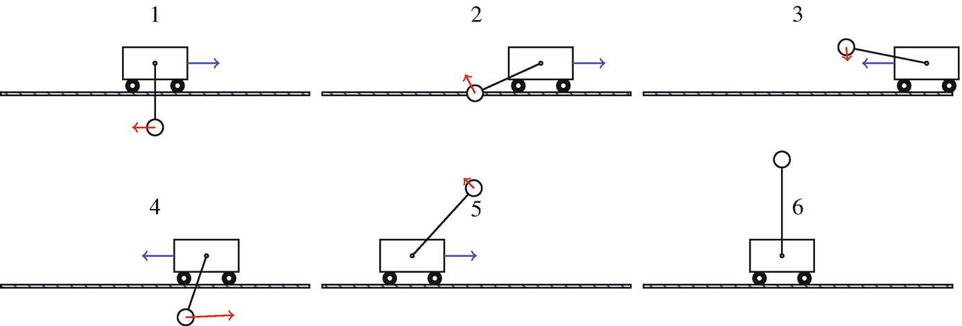
• Learning by Trial and Error.
• No labels needed! Only a Reward Signal.
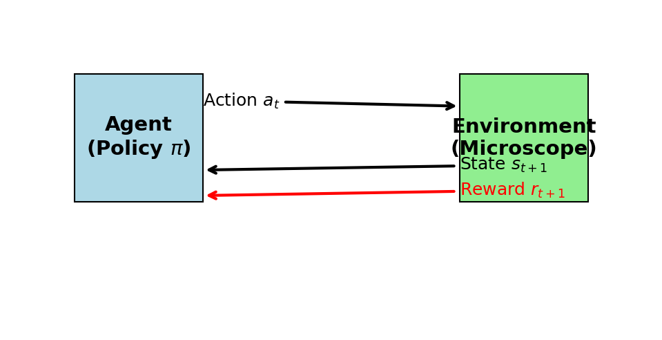
• Agent (ML Model) \(\leftrightarrow\) Environment (The Microscope).

Key Components: State, Action, Reward

• State: What the microscope “sees” (current image/signal).
• Action: What the agent “does” (change lens current, move stage).
• Reward: A scalar indicating how “good” the action was.
• Policy \(\pi(s)\): Mapping from state to action.

Policy Gradients (The Strategy)

• (McClarren 9.2)
• Turning decisions into a probability distribution.
• Update the NN to make “good” decisions (high reward) more likely.
• Exploration vs. Exploitation: Trying new things vs. using what works.

04. Automation in Microscopy

Low-Level Automation: Autofocus

• Traditional: Sweep lens current, pick max sharpness.
• ML: Learn to jump directly to optimal focus from a single blurry image.
• Reward: Image sharpness index (Laplacian, FFT high-freq).

Beam Alignment & Stigmation

• Correcting for non-circular beams and tilt.
• Agent learns to adjust deflector currents by observing beam shape.
• ROI Selection: Automatically finding rare features in large samples.

Multi-Modal Data Fusion

• Combining Images (SEM), Spectra (EDS), and Diffraction (EBSD).
• Bayesian Sensor Fusion: Weighting each sensor by its precision.
• A unified material state vector \(z = f(\text{Image}, \text{Spectrum}, \text{EBSD})\).

UMAP for Streaming Anomaly Triage

The recipe.

1. Embed each incoming SEM / micrograph frame with the lab’s CNN or DINOv2 feature extractor.
2. Maintain a frozen reference UMAP (McInnes et al. 2018) of the nominal manifold, built once on a QC-verified set of frames.
3. Project new frames into that fixed UMAP via umap-learn’s .transform() — no retraining at deploy time.
4. Alarm on frames whose 2-D coordinates land \(> \tau\) standard deviations from the nominal centroid, where \(\tau\) is set by held-out nominal validation.
5. Operator dashboards display the live UMAP with a coloured trail — the eye picks up drift before the threshold does.

Why UMAP and not t-SNE.

• UMAP preserves global structure — clusters of different defect types stay separable across runs.
• UMAP is parametric enough to support .transform() on new points; t-SNE cannot project an unseen frame into a fixed embedding.
• Runs in seconds on a 1080Ti for \(\sim 10^4\) frames — cheap enough to recompute the reference monthly.

Trade-off vs the §5-style raw AE-residual anomaly score. UMAP catches novel-cluster anomalies — a new defect morphology that lands far from any nominal cluster. The autoencoder-residual score catches novel-pixel anomalies — local pixel-level departures. Use both: they cover different failure modes. A frame that scores nominal on AE residual but lands in a sparse UMAP region is exactly the case where a new failure mode is emerging.

MFML reference. The UMAP algorithm — fuzzy simplicial sets, cross-entropy on the graph — is in MFML W9. We use the result here.

Anti-pattern. Training the UMAP on the live deployment stream. The whole point is to have a fixed nominal manifold to compare against; refitting on streaming data lets the embedding silently track the drift, defeating the alarm.

Implementation note. Cache the fitted UMAP() object as a pickle alongside the CNN / DINOv2 weights. Version-pin both. A “tool drift after chamber vent” investigation needs the exact UMAP and feature extractor that were live at the time.

05. Case Study: Industrial Glass Cooling

Why Process Control?

• Automation isn’t just for labs; it’s for manufacturing.
• (McClarren Ch 9.4)
• Problem: Cooling rate controls chemical reactions and physical stress.

RL Control Strategy

• Physics: Coupled Radiation and Diffusion PDEs.
• Input: Current Temp, Target Temp (Future).
• Action: Change boundary temperature \(\Delta u\).
• Reward: Inverse of squared difference from target.

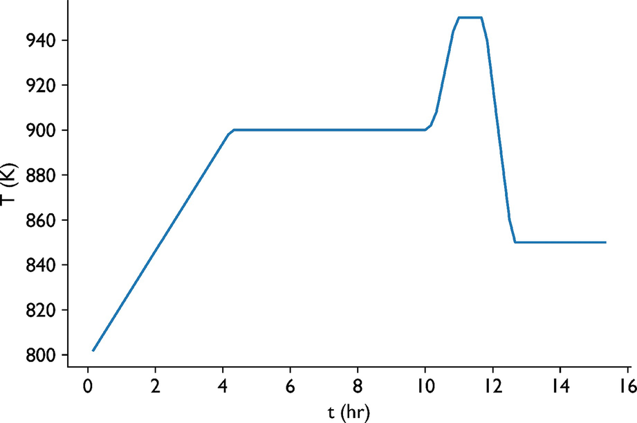
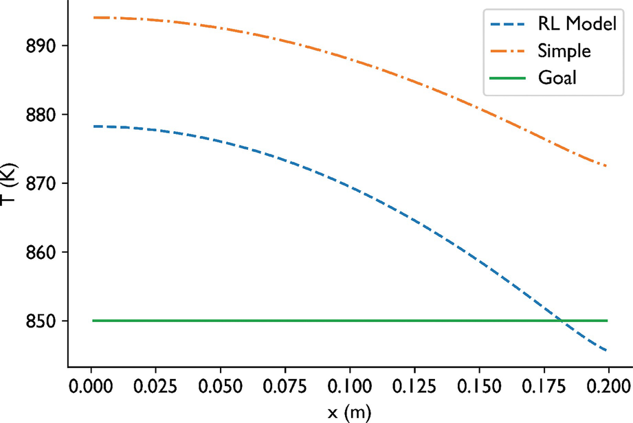
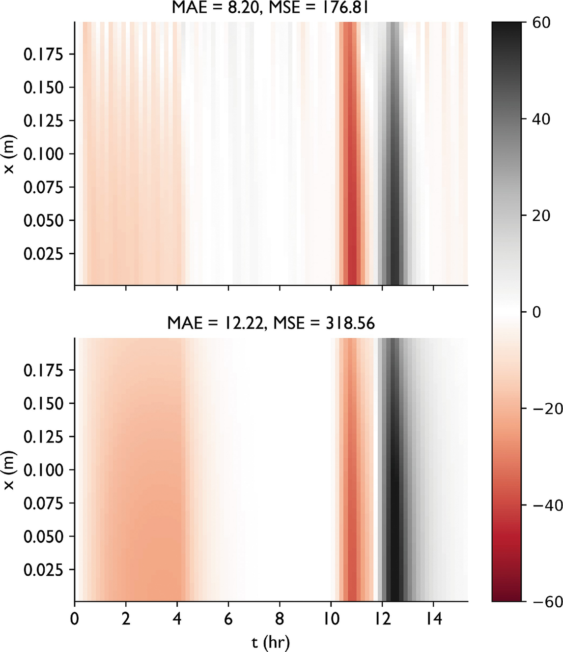
• Outcome: RL learns to “overheat” to reach targets faster, discovering system lags.

06. Synthesis & Self-Driving Labs

The “Self-Driving Lab” Framework

• Automated Synthesis \(\rightarrow\) Automated Characterization \(\rightarrow\) ML Analysis \(\rightarrow\) Loop.
• Integration of Units 1-14.
• Challenges: Software APIs, data standards, and trust.

Conformal Classification — Emit Prediction Sets, Not Single Labels

The recipe (classification variant).

• Train any classifier \(\hat f\) that emits softmax probabilities.
• On a held-out calibration set, compute non-conformity scores

\[s_i = 1 - \hat f_{y_i}(x_i)\]

— one minus the predicted probability of the true class.

• Take \(\hat q = \text{Quantile}_{(1-\alpha)}(s)\).
• At test time, emit the prediction set

\[C(x) = \{\, y : 1 - \hat f_y(x) \le \hat q \,\}.\]

• Guaranteed coverage: the true class lies in \(C(x)\) on at least \(1 - \alpha\) of test inputs (Angelopoulos and Bates 2023).

Why this matters for automated defect detection.

• Instead of class = scratch, the system emits class ∈ {scratch, stain} → send to operator.
• The set size is a calibrated uncertainty signal — singleton sets mean the model is sure, multi-class sets mean it is not.
• Plays cleanly with the §3-style closed-loop triage: singleton set → automate, multi-class set → escalate.

Connection to the U12 split-conformal slide. Unit 11 introduces split conformal for regression (intervals around a point estimate). This slide is the classification variant — same exchangeability argument, score is one-minus-softmax-of-the-true-class, output is a set instead of an interval.

Empty-set degenerate case. If \(1 - \hat f_y(x) > \hat q\) for every class, the prediction set is empty. Rare on calibrated models, but it happens — and it means the input is extreme OOD. Flag and route to human; do not auto-decide.

MFML reference. The exchangeability proof and the finite-sample coverage bound are in MFML W12.

Anti-pattern. Using prediction-set size as the only uncertainty signal. The marginal coverage guarantee is unconditional on the input — a model can satisfy \(\geq 1 - \alpha\) on average while being wildly miscalibrated on individual subgroups (a particular defect class, a particular operator). Always pair with a per-class reliability diagram on a held-out lab-realistic set.

Practical width. On a typical 4-class SEM defect classifier with \(\alpha = 0.1\) and a calibration set of \(\sim 500\) frames, ~70% of test frames get singleton prediction sets (auto), ~25% get 2-class sets (operator-review), ~5% get 3+ class sets (definitely operator). Tune \(\alpha\) to the cost ratio: cheaper operator time → lower \(\alpha\), larger sets, more automation safety.

Recap: Unit 10

• RL is the engine of automation.
• Policy Gradients bridge control and deep learning.
• Reward design is the most critical human task.
• UMAP on a frozen nominal manifold gives streaming anomaly triage; conformal prediction sets turn classifiers into calibrated automate/escalate decisions.
• Next: Handling the “unknown” (Uncertainty and Gaussian Processes).

Continue

• ← Previous: Unit 09b — Transformers for materials (ViT, Flash Attention, Mamba)
• → Next: Unit 11 — Uncertainty-aware regression & Gaussian Processes
• All courses

References & Further Reading

• McClarren (2021): Ch. 9 (Reinforcement Learning)
• Murphy (2012): Ch. 11 (Data Fusion)
• Neuer (2024): Ch. 7.3 (Automation & Causality)
• McInnes, Healy & Melville (2018) — UMAP for streaming anomaly triage (McInnes et al. 2018).
• Angelopoulos & Bates (2023) — conformal prediction sets for automated defect classification (Angelopoulos and Bates 2023).

Angelopoulos, Anastasios N., and Stephen Bates. 2023. “A Gentle Introduction to Conformal Prediction and Distribution-Free Uncertainty Quantification.” Foundations and Trends in Machine Learning 16 (4): 494–591. https://doi.org/10.1561/2200000101.

McInnes, Leland, John Healy, and James Melville. 2018. “UMAP: Uniform Manifold Approximation and Projection for Dimension Reduction.” arXiv Preprint arXiv:1802.03426.

Example Notebook

Week 11: Anomaly Detection via Autoencoder — CahnHilliardDataset

Open rendered notebook →