Machine Learning in Materials Processing & Characterization
Unit 10: ML for Characterization Signals

Prof. Dr. Philipp Pelz

FAU Erlangen-Nürnberg

01. Learning Outcomes

After this unit, you will be able to:

1. Describe the characteristics of 1D characterization signals (XRD, EELS, EDS, XPS, Raman) and why ML is needed

2. Apply PCA to spectral data for dimensionality reduction and denoising

3. Explain the architecture and training of autoencoders and their variants (DAE, CAE, VAE)

4. Compare PCA and autoencoders for spectral compression and feature extraction

5. Design a signal processing pipeline for hyperspectral materials data

02. Beyond Images: 1D Characterization Signals

• Most of our course so far: spatial data (micrographs, microstructure maps)

• But many instruments produce 1D spectral signals:
  • XRD — X-ray Diffraction: crystal structure via Bragg peaks
  • EELS — Electron Energy Loss Spectroscopy: bonding and electronic structure
  • EDS — Energy Dispersive X-ray Spectroscopy: elemental composition
  • XPS — X-ray Photoelectron Spectroscopy: surface chemistry and oxidation states
  • Raman — Vibrational spectroscopy: molecular fingerprints

• Each technique produces a spectrum: intensity vs. energy (or angle, or wavenumber)

• Modern instruments collect millions of spectra per experiment (spectrum imaging)

03. The Nature of Characterization Signals

• High dimensionality: A single spectrum may have 1024, 2048, or 4096 channels
  • Each spectrum is a point in \(\mathbb{R}^{2048}\)

• Sparse peaks: Most channels contain background; only a few contain signal

• Continuous backgrounds: Bremsstrahlung (EDS), plasmon tails (EELS), fluorescence

• Noise: Shot noise (Poisson) dominates at low dose; detector noise adds Gaussian contributions

• Variability: Peak positions shift with composition; peak shapes change with bonding

Spectra as Vectors

A spectrum with \(N\) channels is simply a vector \(\mathbf{x} \in \mathbb{R}^N\). All the linear algebra and ML tools we have learned apply directly — but the physical meaning of each “dimension” (an energy channel) matters for interpretation.

04. The Need for ML

Traditional Analysis Is Breaking Down

• Manual peak fitting is slow, subjective, and does not scale
  • Fitting 10 peaks in 1 spectrum: feasible
  • Fitting 10 peaks in 1,000,000 spectra: impossible

• Overlapping peaks make decomposition ambiguous
  • Fe-L and Mn-L edges in EELS overlap at ~640 eV
  • Ti-K\(\alpha\) and Ba-L\(\alpha\) overlap in EDS at ~4.5 keV

• Subtle spectral changes encode critical physics
  • The Fe-L\(_{2,3}\) edge shape distinguishes Fe\(^{2+}\) from Fe\(^{3+}\)
  • Peak shift of 0.3 eV indicates a change in oxidation state

• Batch effects: Instrument calibration drifts, detector aging, beam damage

05. Goals: Compression, Denoising, Phase ID

Three Core Tasks for ML on Spectra

1. Compression: Reduce \(\mathbf{x} \in \mathbb{R}^{2048}\) to \(\mathbf{z} \in \mathbb{R}^{K}\) with \(K \ll 2048\)
   • Store and transmit massive spectral maps efficiently

2. Denoising: Recover the clean signal from noisy measurements
   • Equivalent to faster acquisition or higher beam current — without the dose

3. Phase Identification: Group similar spectra and identify distinct phases
   • Automated chemical/structural mapping across entire specimens

• All three tasks are connected through dimensionality reduction
• If we find the right low-dimensional representation, compression, denoising, and clustering all follow naturally

Section 2: PCA for Spectra

Eigenspectra, Scree Plots, and Linear Denoising

07. PCA for Spectra

The Classical Tool for Spectral Decomposition (Sandfeld et al. 2024)

• Given \(N\) spectra, each with \(D\) channels, form the data matrix \(\mathbf{X} \in \mathbb{R}^{N \times D}\)

• PCA finds orthogonal directions of maximum variance in this \(D\)-dimensional space

• Each spectrum can be approximated as a linear combination of \(K\) basis vectors:

\[\mathbf{x}_i \approx \bar{\mathbf{x}} + \sum_{k=1}^{K} c_{ik} \, \mathbf{v}_k\]

• \(\bar{\mathbf{x}}\): mean spectrum (average over all \(N\) spectra)
• \(\mathbf{v}_k\): the \(k\)-th eigenvector of the covariance matrix (the \(k\)-th eigenspectrum)
• \(c_{ik}\): the score (coefficient) of spectrum \(i\) on component \(k\)

• Compression: Store only the \(K\) scores \(c_{ik}\) instead of the full \(D\) channels

08. The Basis Function View: Eigenspectra

flowchart LR
    A["Raw Spectrum<br>x ∈ ℝ²⁰⁴⁸"] --> B["Center<br>x - x̄"]
    B --> C["Project onto<br>Eigenspectra V"]
    C --> D["Score Vector<br>c ∈ ℝᴷ"]
    D --> E["Reconstruct<br>x̂ = x̄ + Vc"]
    E --> F["Denoised<br>Spectrum"]

    style A fill:#2d5016,stroke:#4a8c2a,color:#fff
    style D fill:#1a3a5c,stroke:#2a6a9c,color:#fff
    style F fill:#5c1a1a,stroke:#9c2a2a,color:#fff

• The eigenspectra \(\{\mathbf{v}_1, \mathbf{v}_2, \ldots, \mathbf{v}_K\}\) form an orthonormal basis

• Each eigenspectrum is a “building block” — a spectral shape that varies across the dataset

• The scores \(c_{ik} = \mathbf{v}_k^\top (\mathbf{x}_i - \bar{\mathbf{x}})\) are computed by simple inner products

• This is computationally cheap: once the eigenspectra are computed, projecting a new spectrum is a matrix-vector multiply

09. Interpreting Eigenspectra

• PC1 (first eigenspectrum): Typically resembles the mean spectrum
  • Captures the dominant overall shape (background + major peaks)

• PC2, PC3: Capture the dominant variations
  • Often correspond to specific chemical differences between phases
  • Example: PC2 might show positive Fe peaks and negative Cr peaks (Fe vs. Cr variation)

• Higher PCs (\(k > K_{\text{signal}}\)): Capture noise
  • Appear as random oscillations with no physical meaning

10. Intrinsic Dimensionality

• A 2048-channel spectrum lives in \(\mathbb{R}^{2048}\) — but how many dimensions does the data actually use?

• If the sample has 4 distinct phases, the spectra approximately span a 4-dimensional subspace

• The intrinsic dimensionality \(K\) is the number of independent spectral variations

• For most materials datasets: \(K \sim 3\text{--}20 \ll D = 2048\)

Rule of Thumb

The intrinsic dimensionality of a spectral dataset is typically close to the number of distinct phases or chemical environments in the sample, plus a few components for background variations and thickness effects.

11. Scree Plots: Choosing the Number of Components

How Many PCs to Keep? (Sandfeld et al. 2024)

• The scree plot shows the explained variance (eigenvalue) for each component

• Signal components have large eigenvalues; noise components have small, roughly equal eigenvalues

• The Elbow Rule: Keep components before the “elbow” where eigenvalues level off

• Cumulative variance: Often 95% or 99% of total variance is captured by \(K \sim 5\text{--}15\) components

• Alternative: Parallel analysis — compare eigenvalues against those from random data

12. Denoising via Reconstruction

Truncated PCA as a Filter (Sandfeld et al. 2024)

Algorithm:

1. Compute eigenspectra from the dataset: \(\mathbf{V}_K = [\mathbf{v}_1, \ldots, \mathbf{v}_K]\)
2. Project each noisy spectrum: \(\mathbf{c}_i = \mathbf{V}_K^\top (\mathbf{x}_i - \bar{\mathbf{x}})\)
3. Reconstruct: \(\hat{\mathbf{x}}_i = \bar{\mathbf{x}} + \mathbf{V}_K \mathbf{c}_i\)

• The reconstruction \(\hat{\mathbf{x}}_i\) retains only the signal subspace — noise is discarded

• Equivalent to reducing acquisition time by 10x while maintaining chemical sensitivity

13. Think About This…

PCA Denoising: Free Lunch?

Question: If PCA denoising is so effective, why not always reduce acquisition time by 10x and denoise afterwards?

Hint: Think about what happens when a spectrum contains a feature that is unique — present in only one or two pixels of the map.

Consider:

• PCA eigenspectra are computed from the entire dataset
• Rare features may not contribute enough variance to be captured by the top-\(K\) components
• PCA denoising can erase rare phases — minority signals get projected away
• This is a fundamental tension: denoising vs. discovery

Key Insight

PCA denoising is excellent for known, common features but can suppress rare or unexpected signals. Always inspect the residuals \(\mathbf{x}_i - \hat{\mathbf{x}}_i\) for signs of discarded information.

14. PCA Limitations

The Linearity Constraint

• PCA assumes that spectral variations can be expressed as linear combinations
• This works well when: phases mix additively (Beer-Lambert law, EDS from thin sections)

• PCA fails when:
  • Peak positions shift with composition (e.g., XRD peak shift with lattice parameter)
  • Peak shapes change non-linearly (e.g., EELS fine structure with oxidation state)
  • Backgrounds are multiplicative rather than additive

• PCs are orthogonal — but physical phases are not orthogonal
  • PCs can have negative values, but spectra are non-negative
  • Alternative: NMF (Non-negative Matrix Factorization) enforces \(\mathbf{V} \geq 0\), \(\mathbf{C} \geq 0\)

• These limitations motivate autoencoders: non-linear generalizations of PCA

15. Summary: PCA for Spectra

Aspect	PCA
Type	Linear dimensionality reduction
Speed	Very fast (SVD or eigendecomposition)
Solution	Unique, deterministic
Interpretation	Eigenspectra = orthogonal basis functions
Denoising	Truncated reconstruction
Compression	Store \(K\) scores instead of \(D\) channels
Limitation	Cannot handle non-linear variations

When to use PCA:

• As the first step in any spectral analysis pipeline
• When variations are approximately linear (additive mixing)
• When you need fast, reproducible results
• For denoising large spectral maps

Section 3: Autoencoders for Signals

Non-linear Compression, Denoising, and Feature Extraction

17. Autoencoder Concept

A Neural Network That Learns to Compress (Sandfeld et al. 2024)

• An autoencoder (AE) is a neural network trained to reconstruct its own input

• The identity function \(f(\mathbf{x}) = \mathbf{x}\) is trivial — so we add a bottleneck

• The network must learn a compressed representation \(\mathbf{z}\) that captures the essential information

\[\mathbf{z} = f_{\text{enc}}(\mathbf{x}; \theta_{\text{enc}}) \quad \quad \hat{\mathbf{x}} = f_{\text{dec}}(\mathbf{z}; \theta_{\text{dec}})\]

• If \(\dim(\mathbf{z}) \ll \dim(\mathbf{x})\), the AE must discover meaningful features

• With linear activations and one hidden layer, an AE recovers PCA (Sandfeld et al. 2024)
• With non-linear activations, it learns more powerful representations

18. AE Architecture: The Hourglass

flowchart LR
    subgraph Encoder
        I["Input<br>2048 channels"] --> H1["Dense 512<br>ReLU"]
        H1 --> H2["Dense 128<br>ReLU"]
        H2 --> H3["Dense 32<br>ReLU"]
    end

    subgraph Bottleneck
        H3 --> Z["Latent z<br>dim = 8"]
    end

    subgraph Decoder
        Z --> H4["Dense 32<br>ReLU"]
        H4 --> H5["Dense 128<br>ReLU"]
        H5 --> H6["Dense 512<br>ReLU"]
        H6 --> O["Output<br>2048 channels"]
    end

    style I fill:#2d5016,stroke:#4a8c2a,color:#fff
    style Z fill:#8B0000,stroke:#cc3333,color:#fff
    style O fill:#2d5016,stroke:#4a8c2a,color:#fff

• Encoder \(f_{\text{enc}}\): Progressively reduces dimensionality (2048 → 512 → 128 → 32 → 8)

• Bottleneck \(\mathbf{z}\): The latent representation — the “compressed DNA” of the spectrum

• Decoder \(f_{\text{dec}}\): Mirrors the encoder, reconstructing from the latent code (8 → 32 → 128 → 512 → 2048)

19. Why the Bottleneck?

• Without a bottleneck, the network would learn the identity function — trivial and useless

• The bottleneck creates an information bottleneck: the network must decide what to keep and what to discard

• What gets kept: systematic, recurring patterns — peaks, backgrounds, spectral shapes shared across the dataset

• What gets discarded: random, non-repeating variations — noise, detector artifacts, cosmic rays

• The bottleneck size is a hyperparameter:
  • Too large: noise passes through (undercomplete but still noisy)
  • Too small: signal is lost (over-compressed)
  • Just right: captures the intrinsic dimensionality

20. Non-linearity: The Power of AE vs PCA

• PCA: Finds the best linear subspace (a hyperplane)

• AE: Finds the best non-linear manifold (a curved surface)

• Example — XRD peak shift:
  • As lattice parameter \(a\) increases, the (111) peak shifts to lower \(2\theta\)
  • PCA needs multiple components to approximate this shift
  • An AE learns: “one latent variable controls peak position” — direct physical meaning

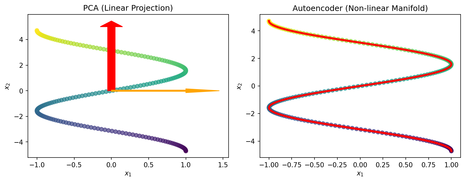
• Non-linearity lets the AE learn physically meaningful latent variables

21. Training: Reconstruction Loss

• The training objective is to minimize the reconstruction error:

\[\mathcal{L}(\theta) = \frac{1}{N} \sum_{i=1}^{N} \|\mathbf{x}_i - \hat{\mathbf{x}}_i\|^2\]

• This is the mean squared error (MSE) between input and output spectra

• Training is unsupervised: no labels needed — the spectrum itself is the target

• Optimization: Adam optimizer, mini-batch gradient descent
• Training on \(10^5\)–\(10^6\) spectra typically takes minutes on a GPU

• Alternative losses:
  • Poisson negative log-likelihood: Better for photon-counting data
  • Spectral angle distance: Focuses on spectral shape, not intensity

22. Latent Space Properties

• The latent variables \(\mathbf{z}\) often develop physically interpretable meanings during training

• Examples of latent-physical correlations:
  • \(z_1 \leftrightarrow\) specimen thickness (controls overall intensity)
  • \(z_2 \leftrightarrow\) Fe/Cr ratio (controls relative peak heights)
  • \(z_3 \leftrightarrow\) oxidation state (controls edge fine structure)

• These correlations are emergent — not programmed, but discovered by the network

• The latent space can be used for:
  • Clustering: Group spectra by latent coordinates
  • Visualization: Plot \(z_1\) vs. \(z_2\) as a chemical map
  • Interpolation: Generate intermediate spectra by moving through latent space

23. Denoising Autoencoders (DAE)

Learning the Clean Manifold (McClarren 2021)

• Standard AE: Input = clean spectrum, Target = clean spectrum
• Denoising AE: Input = noisy spectrum, Target = clean spectrum

\[\mathcal{L}_{\text{DAE}} = \frac{1}{N}\sum_{i=1}^{N} \|\mathbf{x}_i^{\text{clean}} - f_{\text{dec}}(f_{\text{enc}}(\mathbf{x}_i^{\text{clean}} + \boldsymbol{\eta}_i))\|^2\]

• The noise \(\boldsymbol{\eta}_i\) can be:
  • Gaussian: \(\eta \sim \mathcal{N}(0, \sigma^2)\)
  • Poisson: Resample from \(\text{Poisson}(\mathbf{x}_i^{\text{clean}})\)
  • Masking: Randomly zero out spectral channels

• The DAE learns to project noisy spectra back onto the clean data manifold

DAE vs. PCA Denoising

Both discard noise by projecting onto a low-dimensional representation. But a DAE explicitly trains on noisy-clean pairs, making it more robust when the noise model is known. PCA denoising is implicit — it assumes noise is in the discarded components.

24. DAE Example: EELS Spectra

Denoising the Fe-L\(_{2,3}\) Edge

• Problem: At low dose, the EELS fine structure that distinguishes Fe\(^{2+}\) from Fe\(^{3+}\) is buried in noise

• Approach:
  1. Train a DAE on simulated Fe-L edge spectra with known oxidation states
  2. Add Poisson noise at realistic dose levels during training
  3. Apply trained DAE to experimental spectra pixel-by-pixel

• Result: Clear Fe\(^{2+}\)/Fe\(^{3+}\) discrimination at 10x lower dose than conventional analysis

25. Convolutional Autoencoders for Spectra

• Standard AEs use fully connected (dense) layers — every channel connects to every neuron

• Problem: Dense layers do not know that nearby channels are related

• 1D Convolutional AE: Replace dense layers with 1D convolution + pooling

• Advantages:
  • Shift invariance: A peak at 640 eV is recognized the same way as at 650 eV
  • Fewer parameters: Weight sharing across the spectral axis
  • Local feature detection: Learns peak shapes, edge onsets, and local patterns

• Architecture: Input → [Conv1D → ReLU → MaxPool1D] × 3 → Latent → [ConvTranspose1D → ReLU] × 3 → Output

• Particularly effective for XRD and Raman where peak shapes are well-defined

26. Variational Autoencoders (VAE)

• Standard AE: The latent space \(\mathbf{z}\) has no structure — just whatever the network finds useful

• VAE: The encoder outputs a probability distribution \(q(\mathbf{z}|\mathbf{x}) = \mathcal{N}(\boldsymbol{\mu}, \boldsymbol{\sigma}^2)\)

• Training loss adds a KL divergence term:

\[\mathcal{L}_{\text{VAE}} = \underbrace{\|\mathbf{x} - \hat{\mathbf{x}}\|^2}_{\text{reconstruction}} + \beta \cdot \underbrace{D_{\text{KL}}(q(\mathbf{z}|\mathbf{x}) \| p(\mathbf{z}))}_{\text{regularization}}\]

• The KL term encourages the latent space to be smooth and continuous
  • Nearby points in latent space produce similar spectra
  • You can sample from the latent space to generate new, realistic spectra

• Materials application: Generate synthetic training spectra, explore phase space, uncertainty estimation

27. PCA vs. Autoencoder: Head-to-Head

Feature	PCA	Autoencoder
Linearity	Linear only	Non-linear
Speed	Very fast (SVD)	Slower (GPU training)
Solution	Unique, deterministic	Depends on initialization
Interpretability	Eigenspectra are intuitive	Latent space needs probing
Data requirement	Works with small datasets	Needs more data
Peak shifts	Needs many components	Handles naturally
Denoising	Truncated reconstruction	DAE with noise model
Generative	No	Yes (VAE)

Practical recommendation:

• Start with PCA — it is fast, unique, and gives you a baseline
• Switch to AE when PCA reconstruction error plateaus or non-linear effects are important
• Use DAE when you have a good noise model
• Use VAE when you need generative capabilities or uncertainty

28. Think About This…

The Latent Space as a Chemical Compass

Question: You train an autoencoder with a 2D latent space on EDS spectra from a ternary alloy (Fe-Cr-Ni). You plot the latent coordinates for each pixel and color them by known composition. What do you expect to see?

Hint: The alloy has three independent compositional degrees of freedom, but they sum to 100%.

Consider:

• Three elements with the constraint \(c_{\text{Fe}} + c_{\text{Cr}} + c_{\text{Ni}} = 1\) means two independent compositional variables
• A 2D latent space should be sufficient to capture this variation
• You would expect the latent space to look like a triangle (the ternary phase diagram!)
• The autoencoder has rediscovered the Gibbs triangle — without being told anything about thermodynamics

• Follow-up: What if you used a 1D latent space? What would be lost?

29. Anomaly Detection with Autoencoders

• Train the AE on “normal” spectra from the expected phases

• For a new spectrum \(\mathbf{x}\), compute the reconstruction error: \(e = \|\mathbf{x} - \hat{\mathbf{x}}\|^2\)

• If \(e > \tau\) (threshold), the spectrum is anomalous — it does not fit the learned representation

• Materials applications:
  • Detecting unexpected phases or contamination
  • Flagging instrument malfunctions (detector artifacts, calibration drift)
  • Finding rare events (nano-precipitates, grain boundary segregation)

• Unlike supervised anomaly detection, this requires no labels — only knowledge of what “normal” looks like

30. Summary: Autoencoders for Spectra

• Autoencoders are the non-linear generalization of PCA for spectral data

• Key variants:
  • Standard AE: Compression and feature extraction
  • DAE: Denoising with explicit noise models
  • CAE: 1D convolutions for shift-invariant peak detection
  • VAE: Probabilistic latent space for generation and uncertainty

• The latent space is the central concept — it provides:
  • A compressed representation for storage
  • A denoised representation for analysis
  • A feature space for clustering and classification
  • A basis for anomaly detection

• Best practice: Always compare AE results against PCA as a baseline

Section 4: Practical Signal Processing

Pipelines, Hyperspectral Data, and Transfer Learning

32. Signal Processing Workflow

flowchart TD
    A["Raw Spectra<br>(N × D)"] --> B["Preprocessing"]
    B --> B1["Background Subtraction"]
    B --> B2["Normalization"]
    B --> B3["Alignment / Calibration"]
    B1 & B2 & B3 --> C["Dimensionality Reduction"]
    C --> C1["PCA"]
    C --> C2["Autoencoder"]
    C1 & C2 --> D["Latent Representation<br>(N × K)"]
    D --> E1["Clustering<br>(Phase Maps)"]
    D --> E2["Anomaly Detection<br>(Rare Phases)"]
    D --> E3["Classification<br>(Known Phases)"]

    style A fill:#2d5016,stroke:#4a8c2a,color:#fff
    style D fill:#1a3a5c,stroke:#2a6a9c,color:#fff
    style E1 fill:#5c1a1a,stroke:#9c2a2a,color:#fff
    style E2 fill:#5c1a1a,stroke:#9c2a2a,color:#fff
    style E3 fill:#5c1a1a,stroke:#9c2a2a,color:#fff

• Preprocessing: Prepare spectra for ML (remove artifacts, normalize, align)

• Dimensionality Reduction: PCA or AE to extract the latent representation

• Downstream Analysis: Clustering, anomaly detection, or classification in latent space

33. Normalization Strategies

Why Normalize?

• Raw spectral intensities depend on dose, dwell time, specimen thickness — not just chemistry
• Without normalization, PCA/AE will learn intensity variations, not chemical variations

Common Strategies

1. Total-count normalization: \(\mathbf{x}' = \mathbf{x} / \sum_j x_j\)
   • Makes all spectra have unit area — removes thickness/dose effects

2. Peak-height normalization: \(\mathbf{x}' = \mathbf{x} / \max_j x_j\)
   • Makes the strongest peak equal to 1 — preserves relative peak ratios

3. Standard Normal Variate (SNV): \(\mathbf{x}' = (\mathbf{x} - \bar{x}) / s_x\)
   • Centers and scales each spectrum individually — common in chemometrics

4. Min-max per channel: Normalize each energy channel across the dataset
   • Ensures all channels contribute equally to the loss

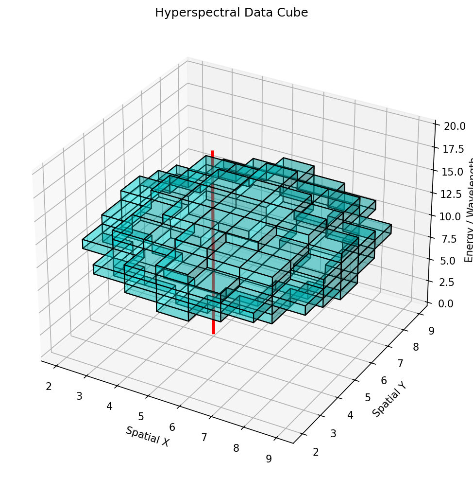
34. Multi-Spectral and Hyperspectral Data

The Data Cube: \((x, y, E)\)

• In spectrum imaging, every pixel \((x, y)\) has an associated spectrum \(\mathbf{s}(E)\)

• The result is a 3D data cube: two spatial dimensions + one spectral dimension

• Typical sizes:
  • STEM-EDS: \(256 \times 256\) pixels \(\times\) \(2048\) channels \(= 134\) million values
  • STEM-EELS: \(100 \times 100\) pixels \(\times\) \(1024\) channels \(= 10\) million values

• Naive approach: Unfold to a \(N_{\text{pixels}} \times D_{\text{channels}}\) matrix, apply PCA/AE per spectrum
• Better approach: Exploit spatial correlations — neighboring pixels likely have similar spectra

35. Spatial-Spectral Autoencoders

• Idea: Use spatial context to improve spectral analysis

• Architecture: Instead of encoding a single spectrum \(\mathbf{x}(x,y)\), encode a patch of spectra around each pixel
  • Input: \(P \times P \times D\) (e.g., \(5 \times 5 \times 2048\))
  • Use 3D convolutions or factored 2D spatial + 1D spectral convolutions

• Benefits:
  • Neighboring pixels provide implicit averaging (denoising)
  • Spatial context helps distinguish interface regions from bulk phases
  • Can learn spatially correlated features (e.g., core-shell structures)

• Trade-off: Spatial smoothing can blur sharp interfaces — choose patch size carefully

36. Learning the Peak Dictionary: End-Members

• Goal: Decompose every spectrum as a non-negative mixture of “pure” end-member spectra

\[\mathbf{x}_i \approx \sum_{k=1}^{K} a_{ik} \, \mathbf{e}_k, \quad a_{ik} \geq 0, \quad \mathbf{e}_k \geq 0\]

• This is Non-negative Matrix Factorization (NMF) — physically more meaningful than PCA
• End-members \(\mathbf{e}_k\) resemble actual spectra of pure phases

• Autoencoder variant: The decoder weights, if constrained to be non-negative, act as a learned dictionary of end-member spectra

• Advantage over database matching: Learns end-members from the data — accounts for instrument-specific peak shapes and backgrounds

37. Signal Separation: Unmixing Overlapping Peaks

• Problem: At a grain boundary between phase A and phase B, the measured spectrum is a mixture

• Linear unmixing: \(\mathbf{x} = \alpha \, \mathbf{e}_A + (1-\alpha) \, \mathbf{e}_B + \boldsymbol{\eta}\)
  • Estimate \(\alpha\) from the latent space position

• Non-linear unmixing: When mixing is not additive
  • Multiple scattering in EELS
  • Absorption effects in thick EDS specimens
  • Autoencoders handle this naturally through non-linear decoder

• Application: Sub-pixel composition mapping
  • Even when the beam probe is larger than the feature, unmixing recovers fractional compositions

38. Transfer Learning for Signals: Synthetic to Real

• Problem: Real spectral datasets for training may be scarce or lack ground truth labels

• Solution: Pre-train on simulated spectra, fine-tune on real data

• Simulation tools:
  • XRD: CrystalDiffract, VESTA, Rietveld simulation
  • EELS: FEFF, DFT-based calculations
  • EDS: Monte Carlo (CASINO, DTSA-II)

• Pipeline:
  1. Simulate spectra for all expected phases with realistic parameters
  2. Add synthetic noise (Poisson + readout noise)
  3. Pre-train DAE or classifier on simulated data
  4. Fine-tune on a small number of real experimental spectra

• Key: The simulation must capture the relevant physics — peak shapes, backgrounds, artifacts

39. Robustness to Instrumental Shifts

• Real instruments are not perfectly stable:
  • Energy calibration drift (peak positions shift over time)
  • Gain changes (detector sensitivity varies)
  • Contamination buildup (affects background)

• A model trained on Monday’s data may fail on Friday’s data

• Strategies for robustness:

1. Data augmentation: During training, randomly shift, scale, and broaden spectra

2. Calibration layer: Learn an alignment transformation as part of the model

3. Domain adaptation: Align feature distributions between source and target instruments

4. Convolutional architectures: Inherently more robust to small shifts (shift equivariance)

40. Summary: Signal Processing Pipeline

Stage	Method	Purpose
Preprocessing	Normalization, alignment	Remove instrumental effects
Reduction	PCA or AE	Compress to latent representation
Denoising	Truncated PCA or DAE	Remove noise while preserving signal
Decomposition	NMF or constrained AE	Identify end-member spectra
Clustering	K-means, UMAP in latent space	Map spatial phase distribution
Anomaly detection	Reconstruction error	Flag unexpected features

41. Non-Negative Matrix Factorization (NMF)

The Natural Choice for Spectra

Constraint: Spectra \(\mathbf{X}\) and their components must be non-negative:

\[\mathbf{X} \approx \mathbf{W}\mathbf{H} \quad \text{s.t. } W_{ik}, H_{kj} \ge 0\]

Matrix	Characterization Meaning
\(\mathbf{X}\) (\(N \times D\))	Raw dataset (spatial pixels \(\times\) energy channels)
\(\mathbf{W}\) (\(N \times K\))	Abundance maps (spatial distribution of each phase)
\(\mathbf{H}\) (\(K \times D\))	End-member spectra (pure phase signatures)

Why NMF beats PCA for spectra:

• Interpretability: Components (H) are “real” spectra, not abstract “variations”
• Physicality: No negative concentrations or negative photon counts
• Parts-based: Naturally learns additive “building blocks” of the signal

Key takeaways:

• The latent space is the universal interface between raw spectra and scientific insight
• Choose the right normalization for your data type
• Always validate against known references and physical expectations

Section 5: Case Studies

From XRD Phase ID to Real-time Signal Monitoring

42. Case Study: Automatic XRD Phase Identification

Problem

• Given a noisy XRD pattern, identify which crystallographic phases are present
• Traditional: Match peaks against the ICDD database (manual, slow, error-prone for mixtures)

ML Approach

1. Train an autoencoder on simulated XRD patterns for all candidate phases
2. Encode the unknown pattern into latent space
3. Use nearest-neighbor classification or clustering in latent space

Results

• Handles multi-phase mixtures by decomposition in latent space
• Robust to preferred orientation and peak broadening (which confuse database matching)
• Can detect amorphous phases as anomalies (high reconstruction error)

43. Case Study: EELS Spectrum Imaging — Fe\(^{2+}\)/Fe\(^{3+}\) Mapping

Problem

• Map the spatial distribution of iron oxidation states at nanometer resolution
• The Fe-L\(_{2,3}\) white line ratio (\(L_3/L_2\)) and onset energy differ between Fe\(^{2+}\) and Fe\(^{3+}\)

ML Approach

• Train a denoising autoencoder on simulated Fe-L edges for both oxidation states
• Apply to experimental EELS spectrum image pixel by pixel
• Use the latent space to map oxidation state continuously (not just binary classification)

Impact

• Enables oxidation state mapping at 5x lower dose than conventional analysis
• Captures continuous gradients (e.g., mixed-valence regions at interfaces)
• Validated against reference spectra from known Fe\(^{2+}\) and Fe\(^{3+}\) standards

44. Case Study: Large-Scale EDS Maps

The Scale Challenge

• Modern SEM/STEM-EDS: \(512 \times 512\) pixels, 2048 channels = ~500,000 spectra
• Multiple fields of view → millions of spectra per sample

PCA-Based Pipeline

1. Apply PCA to the unfolded data cube (\(N \times D\) matrix)
2. Denoise: Reconstruct using top-\(K\) components (typically \(K = 10\text{--}20\))
3. Cluster in score space using K-means
4. Map cluster assignments back to spatial coordinates → phase map

Results

• Denoised maps reveal trace elements below the raw noise floor
• Phase maps identify 5-8 distinct phases automatically
• Processing time: Minutes on a standard workstation (PCA is fast!)

45. Clustering in Latent Space: UMAP Visualization

From Latent Codes to Phase Maps (Sandfeld et al. 2024)

• After dimensionality reduction (PCA or AE), each spectrum is a point \(\mathbf{z}_i \in \mathbb{R}^K\)

• UMAP (Uniform Manifold Approximation and Projection) projects \(K\)-dimensional latent codes to 2D for visualization
  • Preserves both local and global structure (better than t-SNE for this)

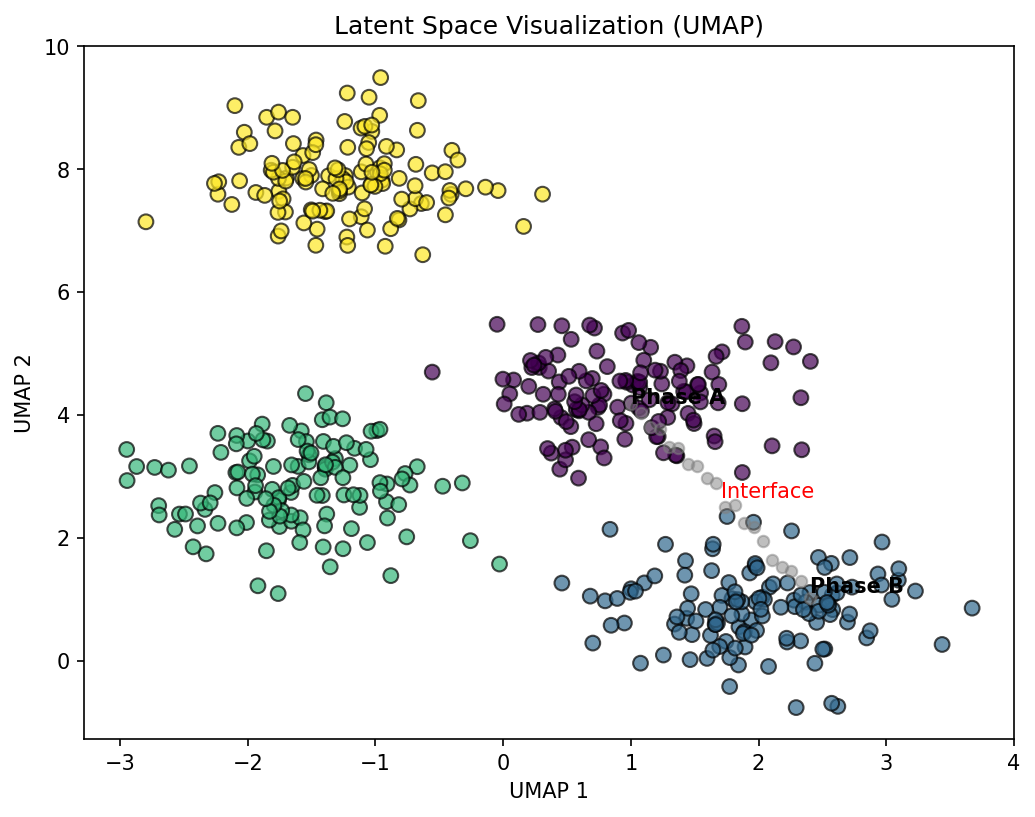
• Clusters in UMAP space correspond to distinct material phases
• Bridges between clusters indicate transition regions (interfaces, diffusion zones)
• Outliers flag anomalies or rare phases

46. Discovering New Phases with Anomaly Detection

When the Model Says “I Don’t Know”

• Train an autoencoder on spectra from known phases
• Apply it to a new sample — most spectra reconstruct well

• High reconstruction error pixels indicate spectra that differ from all known phases

• Discovery workflow:
  1. Map reconstruction error spatially → anomaly map
  2. Extract spectra from high-error regions
  3. Inspect these spectra manually → identify the unknown phase
  4. Add to the training set and retrain

• Example: Discovery of an unexpected intermetallic compound at a diffusion couple interface
  • The AE was trained on the two base metals
  • High reconstruction error at the interface revealed a third phase

47. Real-time Signal Monitoring

Closing the Loop: ML During Acquisition

• Conventional workflow: Acquire → Store → Analyze offline
• ML-enabled workflow: Acquire → Analyze in real time → Adjust acquisition

• Applications:
  • Monitor reconstruction error during scanning — stop early when all phases are mapped
  • Detect beam damage by tracking spectral changes in real time
  • Adaptive acquisition: Spend more time on interesting regions, less on uniform areas

• Requirements:
  • Model must be fast enough for real-time inference (PCA: trivially fast; small AE: ~ms per spectrum)
  • Must handle streaming data (incremental PCA, online AE updates)

The Future Is Adaptive

Combining real-time ML with instrument control creates self-driving microscopes that autonomously explore materials, guided by the scientific questions encoded in the ML model. This is the topic of Unit 11.

48. Exercise Preview

Hands-on: PCA and Autoencoder for EDS Spectra

Part 1: PCA Analysis

1. Load a simulated EDS spectrum image (100 \(\times\) 100 pixels, 1024 channels, 3 phases)
2. Compute PCA and plot the scree plot — determine the intrinsic dimensionality
3. Reconstruct the data using \(K = 3, 5, 10\) components — compare denoised spectra
4. Plot PCA score maps and identify the three phases

Part 2: Autoencoder

5. Build a fully-connected autoencoder with bottleneck size 4
6. Train on the same dataset — compare reconstruction loss vs. PCA
7. Visualize the latent space and compare clustering to PCA scores
8. Introduce an “unknown” phase in a few pixels — use reconstruction error to detect it

Part 3: Denoising

9. Add Poisson noise at various dose levels — compare PCA and DAE denoising

49. Summary and Key Takeaways

What We Learned Today

1. Characterization signals (XRD, EELS, EDS, XPS, Raman) are high-dimensional but lie on low-dimensional manifolds

2. PCA provides fast, linear dimensionality reduction — excellent for denoising and compression, but limited to linear variations

3. Autoencoders extend PCA to non-linear settings — handling peak shifts, shape changes, and complex backgrounds

4. Denoising autoencoders explicitly learn to map noisy spectra to clean ones — enabling lower-dose characterization

5. The latent space is the universal interface: it enables compression, denoising, clustering, anomaly detection, and visualization

6. Practical pipelines require careful normalization, validation, and robustness to instrumental shifts

Next unit: Unit 11 — Automation in Microscopy (closing the loop)

50. References

Core References

• Sandfeld et al. (2024): Ch. 15 (PCA), Ch. 15.3.2 (Scree Plots), Ch. 15.3.3 (Denoising), Ch. 15.6 (Clustering), Ch. 19.4 (Autoencoders)
• McClarren (2021): Ch. 8.3.2 (Denoising Autoencoders)
• Neuer et al. (2024): Ch. 5 (Unsupervised Learning)

Further Reading

• Kingma & Welling (2014): “Auto-Encoding Variational Bayes” — the original VAE paper
• Lee & Seung (1999): “Learning the parts of objects by non-negative matrix factorization” — NMF
• McInnes et al. (2018): “UMAP: Uniform Manifold Approximation and Projection” — dimensionality reduction for visualization

Software

• HyperSpy: Open-source Python library for multi-dimensional spectral data analysis
• scikit-learn: PCA, NMF, K-means implementations
• PyTorch / TensorFlow: Autoencoder implementations

McClarren, Ryan G. 2021. Machine Learning for Engineers: Using Data to Solve Problems for Physical Systems. Springer.

Neuer, Michael et al. 2024. Machine Learning for Engineers: Introduction to Physics-Informed, Explainable Learning Methods for AI in Engineering Applications. Springer Nature.

Sandfeld, Stefan et al. 2024. Materials Data Science. Springer.